Unimodal distribution

The following example demonstrates the statistical learning based determination of the nuclear shielding tensor parameters from a one-dimensional cross-section of a magic-angle flipping (MAF) spectrum. In this example, we use a synthetic MAF lineshape from a unimodal tensor distribution.

Before getting started

Import all relevant packages.

import csdmpy as cp
import matplotlib.pyplot as plt
import numpy as np

from mrinversion.kernel.nmr import ShieldingPALineshape
from mrinversion.linear_model import SmoothLasso, SmoothLassoCV, TSVDCompression
from mrinversion.utils import get_polar_grids

# Setup for the matplotlib figures


# function for 2D x-y plot.
def plot2D(ax, csdm_object, title=""):
    # convert the dimension coordinates of the csdm_object from Hz to pmm.
    _ = [item.to("ppm", "nmr_frequency_ratio") for item in csdm_object.dimensions]

    levels = (np.arange(9) + 1) / 10
    plt.figure(figsize=(4.5, 3.5))
    ax.contourf(csdm_object, cmap="gist_ncar", levels=levels)
    ax.grid(None)
    ax.set_title(title)
    get_polar_grids(ax)
    ax.set_aspect("equal")

Dataset setup

Import the dataset

Load the dataset. Here, we import the dataset as a CSDM data-object.

# the 1D MAF cross-section data in csdm format
filename = "https://osu.box.com/shared/static/puxfgdh25rru1q3li124anylkgup8rdp.csdf"
data_object = cp.load(filename)

# convert the data dimension from `Hz` to `ppm`.
data_object.dimensions[0].to("ppm", "nmr_frequency_ratio")

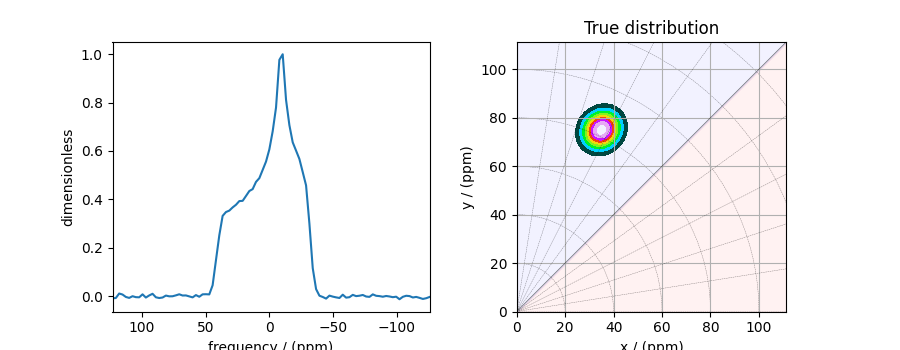
The variable data_object holds the 1D MAF cross-section. For comparison, let’s also import the true tensor parameter distribution from which the synthetic 1D pure anisotropic MAF cross-section line-shape is simulated.

datafile = "https://osu.box.com/shared/static/s5wpm26w4cv3w64qjhouqu458ch4z0nd.csdf"
true_data_object = cp.load(datafile)

The plot of the 1D MAF cross-section along with the 2D true tensor parameter distribution of the synthetic dataset is shown below.

# the plot of the 1D MAF cross-section dataset.
_, ax = plt.subplots(1, 2, figsize=(9, 3.5), subplot_kw={"projection": "csdm"})
ax[0].plot(data_object)
ax[0].invert_xaxis()

# the plot of the true tensor distribution.
plot2D(ax[1], true_data_object, title="True distribution")
plt.tight_layout()
plt.show()

• 
• 

Linear Inversion setup

Dimension setup

Anisotropic-dimension: The dimension of the dataset that holds the pure anisotropic frequency contributions, which in this case, is the only dimension.

anisotropic_dimension = data_object.dimensions[0]

x-y dimensions: The two inverse dimensions corresponding to the x and y-axis of the x-y grid.

inverse_dimension = [
    cp.LinearDimension(count=25, increment="370 Hz", label="x"),  # the `x`-dimension.
    cp.LinearDimension(count=25, increment="370 Hz", label="y"),  # the `y`-dimension.
]

Generating the kernel

For MAF datasets, the line-shape kernel corresponds to the pure nuclear shielding anisotropy line-shapes. Use the ShieldingPALineshape class to generate a shielding line-shape kernel.

lineshape = ShieldingPALineshape(
    anisotropic_dimension=anisotropic_dimension,
    inverse_dimension=inverse_dimension,
    channel="29Si",
    magnetic_flux_density="9.4 T",
    rotor_angle="90 deg",
    rotor_frequency="14 kHz",
    number_of_sidebands=4,
)

Here, lineshape is an instance of the ShieldingPALineshape class. The required arguments of this class are the anisotropic_dimension, inverse_dimension, and channel. We have already defined the first two arguments in the previous sub-section. The value of the channel argument is the nucleus observed in the MAF experiment. In this example, this value is ‘29Si’. The remaining arguments, such as the magnetic_flux_density, rotor_angle, and rotor_frequency, are set to match the conditions under which the spectrum was acquired. The value of the number_of_sidebands argument is the number of sidebands calculated for each line-shape within the kernel.

Once the ShieldingPALineshape instance is created, use the kernel() method of the instance to generate the MAF line-shape kernel.

K = lineshape.kernel(supersampling=1)

Data Compression

Data compression is optional but recommended. It may reduce the size of the inverse problem and, thus, further computation time.

new_system = TSVDCompression(K, data_object)
compressed_K = new_system.compressed_K
compressed_s = new_system.compressed_s

print(f"truncation_index = {new_system.truncation_index}")

Out:

compression factor = 1.5737704918032787
truncation_index = 61

Solving the inverse problem

Smooth-LASSO problem

Solve the smooth-lasso problem. You may choose to skip this step and proceed to the statistical learning method. Usually, the statistical learning method is a time-consuming process that solves the smooth-lasso problem over a range of predefined hyperparameters. If you are unsure what range of hyperparameters to use, you can use this step for a quick look into the possible solution by giving a guess value for the \(\alpha\) and \(\lambda\) hyperparameters, and then decide on the hyperparameters range accordingly.

# guess alpha and lambda values.
s_lasso = SmoothLasso(alpha=5e-5, lambda1=5e-6, inverse_dimension=inverse_dimension)
s_lasso.fit(K=compressed_K, s=compressed_s)
f_sol = s_lasso.f

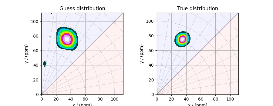
Here, f_sol is the solution corresponding to hyperparameters \(\alpha=5\times10^{-5}\) and \(\lambda=5\times 10^{-6}\). The plot of this solution is

_, ax = plt.subplots(1, 2, figsize=(9, 3.5), subplot_kw={"projection": "csdm"})

# the plot of the guess tensor distribution solution.
plot2D(ax[0], f_sol / f_sol.max(), title="Guess distribution")

# the plot of the true tensor distribution.
plot2D(ax[1], true_data_object, title="True distribution")
plt.tight_layout()
plt.show()

• 
• 
• 

Predicted spectrum

You may also evaluate the predicted spectrum from the above solution following

residuals = s_lasso.residuals(K, data_object)
predicted_spectrum = data_object - residuals

plt.figure(figsize=(4, 3))
plt.subplot(projection="csdm")
plt.plot(data_object, color="black", label="spectrum")  # the original spectrum
plt.plot(predicted_spectrum, color="red", label="prediction")  # the predicted spectrum
plt.gca().invert_xaxis()
plt.legend()
plt.tight_layout()
plt.show()

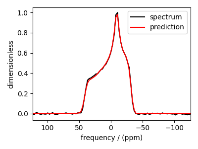
As you can see from the predicted spectrum, our guess isn’t far from the optimum hyperparameters. Let’s create a search grid about the guess hyperparameters and run a cross-validation method for selection.

Statistical learning of the tensors

Smooth LASSO cross-validation

Create a guess range of values for the \(\alpha\) and \(\lambda\) hyperparameters. The following code generates a range of \(\lambda\) and \(\alpha\) values that are uniformly sampled on the log scale.

lambdas = 10 ** (-5.2 - 1 * (np.arange(6) / 5))
alphas = 10 ** (-4 - 2 * (np.arange(6) / 5))

# set up cross validation smooth lasso method
s_lasso_cv = SmoothLassoCV(
    alphas=alphas,
    lambdas=lambdas,
    inverse_dimension=inverse_dimension,
    sigma=0.005,
    folds=10,
)
# run the fit using the compressed kernel and compressed signal.
s_lasso_cv.fit(compressed_K, compressed_s)

The optimum hyper-parameters

Use the hyperparameters attribute of the instance for the optimum hyper-parameters, \(\alpha\) and \(\lambda\), determined from the cross-validation.

print(s_lasso_cv.hyperparameters)

Out:

{'alpha': 6.30957344480193e-06, 'lambda': 1.584893192461114e-06}

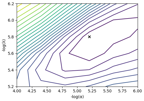
The cross-validation surface

Optionally, you may want to visualize the cross-validation error curve/surface. Use the cross_validation_curve attribute of the instance, as follows. The cross-validation metric is the mean square error (MSE).

cv_curve = s_lasso_cv.cross_validation_curve

# plot of the cross-validation curve
plt.figure(figsize=(5, 3.5))
ax = plt.subplot(projection="csdm")
ax.contour(np.log10(s_lasso_cv.cross_validation_curve), levels=25)
ax.scatter(
    -np.log10(s_lasso_cv.hyperparameters["alpha"]),
    -np.log10(s_lasso_cv.hyperparameters["lambda"]),
    marker="x",
    color="k",
)
plt.tight_layout(pad=0.5)
plt.show()

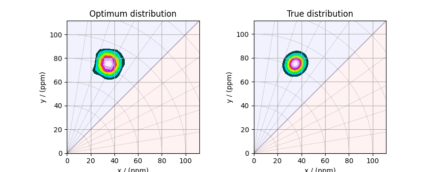
The optimum solution

The f attribute of the instance holds the solution.

f_sol = s_lasso_cv.f

The corresponding plot of the solution, along with the true tensor distribution, is shown below.

_, ax = plt.subplots(1, 2, figsize=(9, 3.5), subplot_kw={"projection": "csdm"})

# the plot of the tensor distribution solution.
plot2D(ax[0], f_sol / f_sol.max(), title="Optimum distribution")

# the plot of the true tensor distribution.
plot2D(ax[1], true_data_object, title="True distribution")
plt.tight_layout()
plt.show()

• 
• 
•