Introduction

Objective

In mrinversion, we solve for the distribution of the second-rank traceless symmetric tensor principal components, through an inversion of a pure anisotropic NMR spectrum.

In the case of the shielding tensors, the pure anisotropic frequency spectra corresponds the cross-sections of the 2D isotropic v.s. anisotropic correlation spectrum, such as the 2D One Pulse (TOP) MAS, phase adjusted spinning sidebands (PASS), magic-angle turning (MAT), extended chemical shift modulation (XCS), magic-angle hopping (MAH), magic-angle flipping (MAF), and Variable Angle Correlation Spectroscopy (VACSY). A key feature of all these 2D isotropic/anisotropic correlation spectra—–either as acquired or after a shear transformation—–is that the anisotropic cross-section can be modeled as a linear combination of subspectra,

(1)\[s(\nu| \delta_\text{iso}) = \int_{\bf R} \mathcal{K}(\nu, {\bf R}) f({\bf R} | \delta_\text{iso}) d{\bf R},\]

where \(s(\nu| \delta_\text{iso})\) is the observed anisotropic cross-section at a given isotropic shift, \(\delta_\text{iso}\), \(\mathcal{K}(\nu, {\bf R})\) represents a simulated subspectrum of a nuclear spin system with a given set of parameters, \({\bf R}\), and \(f({\bf R} | \delta_\text{iso})\) is the probability of the respective set of parameters. In Eq. (1), \({\bf R}\) represents the anisotropic and asymmetry parameters of the shielding tensor.

Note, Eq. (1) is a Fredholm integral of the first kind.

Generic Linear problem

Linear inverse problems on Fredholm integral of the first kind are frequently encountered in the scientific community and have the following generic form

(2)\[ {\bf s} = {\bf K \cdot f},\]

where \({\bf K} \in \mathbb{R}^{m\times n}\) is the transforming kernel (matrix), \({\bf f} \in \mathbb{R}^n\) is the unknown and desired solution, and \({\bf s} \in \mathbb{R}^m\) is the known signal, which includes the measurement noise. When the matrix \({\bf K}\) is non-singular and \(m=n\), the solution to the problem in Eq. (2) has a simple closed-form solution,

(3)\[{\bf f} = {\bf K}^{-1} \cdot {\bf s}.\]

The deciding factor whether the solution \({\bf f}\) exists in Eq. (3) is whether or not the kernel \({\bf K}\) is invertible. Often, most scientific problems with practical applications suffer from singular, near-singular, or ill-conditioned kernels, where \({\bf K}^{-1}\) doesn’t exist. Such types of problems are termed as ill-posed. The inversion of a purely anisotropic NMR spectrum to the distribution of the tensorial parameters is one such ill-posed problem.

Regularized linear problem

A common approach in solving ill-posed problems is to employ the regularization methods of form

(4)\[{\bf f^\dagger} = \underset{{\bf f} > 0}{\text{argmin}} \left( \|{\bf K \cdot f} - {\bf s}\|^2_2 + g({\bf f}) \right),\]

where \(\|{\bf z}\|_2\) is the l-2 norm of \({\bf z}\), \(g({\bf f})\) is the regularization term, and \({\bf f}^\dagger\) is the regularized solution. The choice of the regularization term, \(g({\bf f})\), is often based on prior knowledge of the system for which the linear problem is defined. For anisotropic NMR spectrum inversion, we choose the smooth-LASSO regularization.

Smooth-LASSO regularization

Our prior assumption for the distribution of the tensorial parameters is that it should be smooth and continuous for disordered and sparse and discrete for crystalline materials. Therefore, we employ the smooth-lasso method, which is a linear model that is trained with the combined l1 and l2 priors as the regularizer. The method minimizes the objective function,

(5)\[\| {\bf K \cdot f - s} \|^2_2 + \alpha \sum_{i=1}^{d} \| {\bf J}_i \cdot {\bf f} \|_2^2 + \lambda \| {\bf f} \|_1 ,\]

where \(\alpha\) and \(\lambda\) are the hyperparameters controlling the smoothness and sparsity of the solution \({\bf f}\). The matrix \({\bf J}_i\) typically reflects some underlying geometry or the structure in the true solution. Here, \({\bf J}_i\) is defined to promote smoothness along the \(\text{i}^\text{th}\) dimension of the solution \({\bf f}\) and is given as

(6)\[{\bf J}_i = {\bf I}_{n_1} \otimes \cdots \otimes {\bf A}_{n_i} \otimes \cdots \otimes {\bf I}_{n_{d}},\]

where \({\bf I}_{n_i} \in \mathbb{R}^{n_i \times n_i}\) is the identity matrix, and \({\bf A}_{n_i}\) is the first difference matrix given as

(7)\[\begin{split}{\bf A}_{n_i} = \left(\begin{array}{ccccc} 1 & -1 & 0 & \cdots & \vdots \\ 0 & 1 & -1 & \cdots & \vdots \\ \vdots & \vdots & \vdots & \vdots & 0 \\ 0 & \cdots & 0 & 1 & -1 \end{array}\right) \in \mathbb{R}^{(n_i-1)\times n_i}.\end{split}\]

The symbol \(\otimes\) is the Kronecker product. The terms, \(\left(n_1, n_2, \cdots, n_d\right)\), are the number of points along the respective dimensions, with the constraint that \(\prod_{i=1}^{d}n_i = n\), where \(d\) is the total number of dimensions in the solution \({\bf f}\), and \(n\) is the total number of features in the kernel, \({\bf K}\).

Understanding the x-y plot

A second-rank symmetric tensor, \({\bf S}\), in a three-dimensional space, is described by three principal components, \(s_{xx}\), \(s_{yy}\), and \(s_{zz}\), in the principal axis system (PAS). Often, depending on the context of the problem, the three principal components are expressed with three new parameters following a convention. One such convention is the Haeberlen convention, which defines \(\delta_\text{iso}\), \(\zeta\), and \(\eta\), as the isotropic shift, anisotropy, and asymmetry parameters, respectively. Here, the parameters \(\zeta\) and \(\eta\) contribute to the purely anisotropic frequencies, and determining the distribution of these two parameters is the focus of this library.

Defining the inverse grid

When solving any linear inverse problem, one needs to define an inverse grid before solving the problem. A familiar example is the inverse Fourier transform, where the inverse grid is defined following the Nyquist–Shannon sampling theorem. Unlike inverse Fourier transform, however, there is no well-defined sampling grid for the second-rank traceless symmetric tensor parameters. One obvious choice is to define a two-dimensional \(\zeta\)-\(\eta\) Cartesian grid.

As far as the inversion problem is concerned, \(\zeta\) and \(\eta\) are just labels for the subspectra. In simplistic terms, the inversion problem solves for the probability of each subspectrum, from a given pre-defined basis of subspectra, that describes the observed spectrum. If the subspectra basis is defined over a \(\zeta\)-\(\eta\) Cartesian grid, multiple \((\zeta, \eta)\) coordinates points to the same subspectra. For example, the subspectra from coordinates \((\zeta, \eta=1)\) and \((-\zeta, \eta=1)\) are identical, therefore, distinguishing these coordinates from the subspectra becomes impossible.

The issue of multiple coordinates pointing to the same object is not new. It is a common problem when representing polar coordinates in the Cartesian basis. Try describing the coordinates of the south pole using latitudes and longitudes. You can define the latitude, but describing longitude becomes problematic. A similar situation arises in the context of second-rank traceless tensor parameters when the anisotropy goes to zero. You can specify the anisotropy as zero, but defining asymmetry becomes problematic.

Introducing the \(x\)-\(y\) grid

A simple fix to this issue is to define the \((\zeta, \eta)\) coordinates in a polar basis. We, therefore, introduce a piece-wise polar grid representation of the second-rank traceless tensor parameters, \(\zeta\)-\(\eta\), defined as

(8)\[\begin{split}r_\zeta = | \zeta_ | ~~~~\text{and}~~~~ \theta = \left\{ \begin{array}{l r} \frac{\pi}{4} \eta &: \zeta \le 0, \\ \frac{\pi}{2} \left(1 - \frac{\eta}{2} \right) &: \zeta > 0. \end{array} \right.\end{split}\]

Because Cartesian grids are more manageable in computation, we re-express the above polar piece-wise grid as the x-y Cartesian grid following,

(9)\[x = r_\zeta \cos\theta ~~~~\text{and}~~~~ y = r_\zeta \sin\theta.\]

In the x-y grid system, the basis subspectra are relatively distinguishable. The mrinversion library provides a utility function to render the piece-wise polar grid for your matplotlib figures. Copy-paste the following code in your script.

>>> import matplotlib.pyplot as plt 
>>> from mrinversion.utils import get_polar_grids 
...
>>> plt.figure(figsize=(4, 3.5)) 
>>> ax=plt.gca() 
>>> # add your plots/contours here.
>>> get_polar_grids(ax) 
>>> ax.set_xlabel('x / ppm') 
>>> ax.set_ylabel('y / ppm') 
>>> plt.tight_layout() 
>>> plt.show() 

(png, hires.png, pdf)

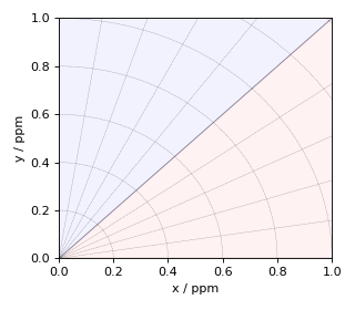
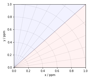
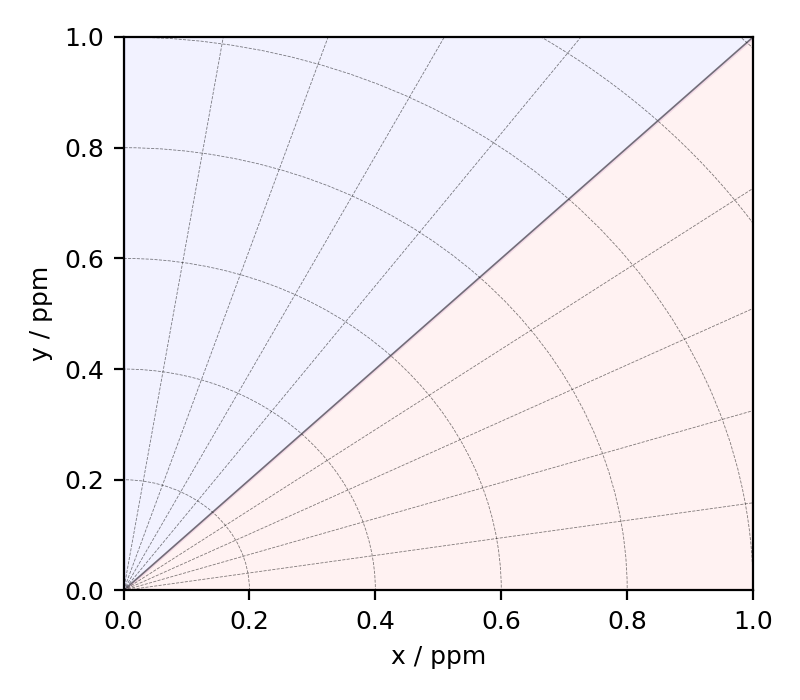
Figure 1 The figure depicts the piece-wise polar \(\zeta\)-\(\eta\) grid represented on an x-y grid. The radial and angular grid lines represent the magnitude of \(\zeta\) and \(\eta\), respectively. The blue and red shading represents the positive and negative values of \(\zeta\), respectively. The radian grid lines are drawn at every 0.2 ppm increments of \(\zeta\), and the angular grid lines are drawn at every 0.2 increments of \(\eta\). The x and y-axis are \(\eta=0\), and the diagonal \(x=y\) is \(\eta=1\).

If you are familiar with the matplotlib library, you may notice that most code lines are the basic matplotlib statements, except for the line that says get_polar_grids(ax). The get_polar_grids() is a utility function that generates the piece-wise polar grid for your figures.

Here, the shielding anisotropy parameter, \(\zeta\), is the radial dimension, and the asymmetry parameter, \(\eta\), is the angular dimension, defined using Eqs. (8) and (9). The region in blue and red corresponds to the positive and negative values of \(\zeta\), where the magnitude of the anisotropy increases radially. The x and the y-axis are \(\eta=0\) for the negative and positive \(\zeta\), respectively. When moving towards the diagonal from x or y-axes, the asymmetry parameter, \(\eta\), uniformly increase, where the diagonal is \(\eta=1\).