Utils
- mrinversion.kernel.utils.x_y_to_zeta_eta(x, y)[source]
Convert the coordinates \((x,y)\) to \((\zeta, \eta)\) using the following definition,
(18)¶\[\begin{split}\left.\begin{array}{rl} \zeta &= \sqrt{x^2 + y^2}, \\ \eta &= \frac{4}{\pi} \tan^{-1} \left| \frac{x}{y} \right| \end{array} {~~~~~~~~} \right\} {~~~~~~~~} |x| \le |y|.\end{split}\](19)¶\[\begin{split}\left.\begin{array}{rl} \zeta &= -\sqrt{x^2 + y^2}, \\ \eta &= \frac{4}{\pi} \tan^{-1} \left| \frac{y}{x} \right| \end{array} {~~~~~~~~} \right\} {~~~~~~~~} |x| > |y|.\end{split}\]- Parameters
x – floats or Quantity object. The coordinate x.
y – floats or Quantity object. The coordinate y.
- Returns
A list of two ndarrays. The first array is the \(\zeta\) coordinates. The second array is the \(\eta\) coordinates.
- mrinversion.kernel.utils.zeta_eta_to_x_y(zeta, eta)[source]
Convert the coordinates \((\zeta,\eta)\) to \((x, y)\) using the following definition,
(20)¶\[\begin{split}\left. \begin{array}{rl} x &= |\zeta| \sin\theta, \\ y &= |\zeta| \cos\theta \end{array} {~~~~~~~~} \right\} {~~~~~~~~} \zeta \ge 0\end{split}\](21)¶\[\begin{split}\left. \begin{array}{rl} x &= |\zeta| \cos\theta, \\ y &= |\zeta| \sin\theta \end{array} {~~~~~~~~} \right\} {~~~~~~~~} \zeta < 0\end{split}\]where \(\theta = \frac{\pi}{4}\eta\).
- Parameters
x – ndarray or list of floats. The coordinate x.
y – ndarray or list of floats. The coordinate y.
- Returns
A list of ndarrays. The first array holds the coordinate \(x\). The second array holds the coordinates \(y\).
- mrinversion.utils.get_polar_grids(ax, ticks=None, offset=0)[source]
Generate a piece-wise polar grid of Haeberlen parameters, zeta and eta.
- Parameters
ax – Matplotlib Axes.
ticks – Tick coordinates where radial grids are drawn. The value can be a list or a numpy array. The default value is None.
offset – The grid is drawn at an offset away from the origin.
- mrinversion.utils.to_Haeberlen_grid(csdm_object, zeta, eta, n=5)[source]
Convert the three-dimensional p(iso, x, y) to p(iso, zeta, eta) tensor distribution.
- Parameters
csdm_object (CSDM) – A CSDM object containing the 3D p(iso, x, y) distribution.
zeta (CSDM.Dimension) – A CSDM dimension object describing the zeta dimension.
eta (CSDM.Dimension) – A CSDM dimension object describing the eta dimension.
n (int) – An interger used in linear interpolation of the data. The default is 5.
- mrinversion.utils.plot_3d(ax, csdm_object, elev=28, azim=-150, x_lim=None, y_lim=None, z_lim=None, max_2d=None, max_1d=None, cmap=<matplotlib.colors.LinearSegmentedColormap object>, box=False, clip_percent=0.0, linewidth=1, alpha=0.15, **kwargs)[source]
Generate a 3D density plot with 2D contour and 1D projections.
- Parameters
ax – Matplotlib Axes to render the plot.
csdm_object – A 3D{1} CSDM object holding the data.
elev – (optional) The 3D view angle, elevation angle in the z plane.
azim – (optional) The 3D view angle, azimuth angle in the x-y plane.
x_lim – (optional) The x limit given as a list, [x_min, x_max].
y_lim – (optional) The y limit given as a list, [y_min, y_max].
z_lim – (optional) The z limit given as a list, [z_min, z_max].
max_2d – (Optional) The normalization factor of the 2D contour projections. The attribute is meaningful when multiple 3D datasets are viewed on the same plot. The value is given as a list, [yz, xz, xy], where ij is the maximum of the projection onto the ij plane, \(i,j \in [x, y, z]\).
max_1d – (Optional) The normalization factor of the 1D projections. The attribute is meaningful when multiple 3D datasets are viewed on the same plot. The value is given as a list, [x, y, z], where i is the maximum of the projection onto the i axis, \(i \in [x, y, z]\).
cmap – (Optional) The colormap used in rendering the volumetric plot. The same colormap is used for the 2D contour projections. For 1D plots, the first color in the colormap scheme is used for the line color.
box – (Optional) If True, draw a box around the 3D data region.
clip_percent – (Optional) The amplitudes of the dataset below the given percent is made transparent for the volumetric plot.
linewidth – (Optional) The linewidth of the 2D countours, 1D plots and box.
alpha – (Optional) The amount of alpha(transparency) applied in rendering the 3D volume.
