Getting started with mrinversion
We have put together a set of guidelines for using the mrinversion package. We encourage our users to follow these guidelines for consistency.
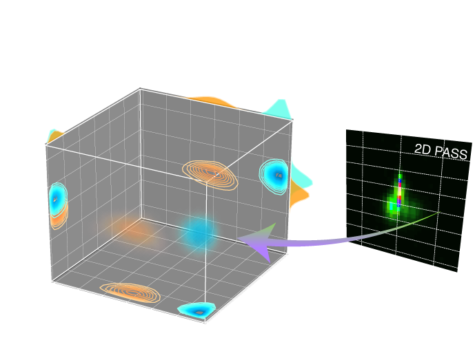
Let’s examine the inversion of a purely anisotropic MAS sideband spectrum into a 2D distribution of nuclear shielding anisotropy parameters. For illustrative purposes, we use a synthetic one-dimensional purely anisotropic spectrum. Think of this as a cross-section of your 2D MAT/PASS dataset.
Import relevant modules
>>> import numpy as np
>>> import matplotlib.pyplot as plt
>>> from matplotlib import rcParams
>>> from mrinversion.utils import get_polar_grids
...
>>> rcParams['pdf.fonttype'] = 42 # for exporting figures as illustrator editable pdf.
...
>>> # a function to plot the 2D tensor parameter distribution
>>> def plot2D(ax, csdm_object, title=''):
...     # convert the dimension from `Hz` to `ppm`.
...     _ = [item.to('ppm', 'nmr_frequency_ratio') for item in csdm_object.dimensions]
...
...     levels = (np.arange(9)+1)/10
...     ax.contourf(csdm_object, cmap='gist_ncar', levels=levels)
...     ax.grid(None)
...     ax.set_title(title)
...     ax.set_aspect("equal")
...
...     # The get_polar_grids method place a polar zeta-eta grid on the background.
...     get_polar_grids(ax)
Import the dataset
The first step is getting the sideband spectrum. In this example, we get the data from a CSDM 1 compliant file-format. Import the csdmpy module and load the dataset as follows,
Note
The CSDM file-format is a new open-source universal file format for multi-dimensional datasets. It is supported by NMR programs such as SIMPSON 2, DMFIT 3, and RMN 4. A python package supporting CSDM file-format, csdmpy, is also available.
>>> import csdmpy as cp
...
>>> filename = "https://osu.box.com/shared/static/xnlhecn8ifzcwx09f83gsh27rhc5i5l6.csdf"
>>> data_object = cp.load(filename) # load the CSDM file with the csdmpy module
Here, the variable data_object is a CSDM object. The NMR spectroscopic dimension is a frequency dimension. NMR spectroscopists, however, prefer to view the spectrum on a dimensionless scale. If the dataset dimension within the CSDM object is in frequency, you may convert it into ppm as follows,
>>> # convert the dimension coordinates from `Hz` to `ppm`.
>>> data_object.dimensions[0].to('ppm', 'nmr_frequency_ratio')
In the above code, we convert the dimension at index 0 from Hz to ppm. For multi-dimensional datasets, use the appropriate indexing to convert individual dimensions to ppm.
For comparison, let’s also include the true probability distribution from which the synthetic spinning sideband dataset is derived.
>>> datafile = "https://osu.box.com/shared/static/lufeus68orw1izrg8juthcqvp7w0cpzk.csdf"
>>> true_data_object = cp.load(datafile) # the true solution for comparison
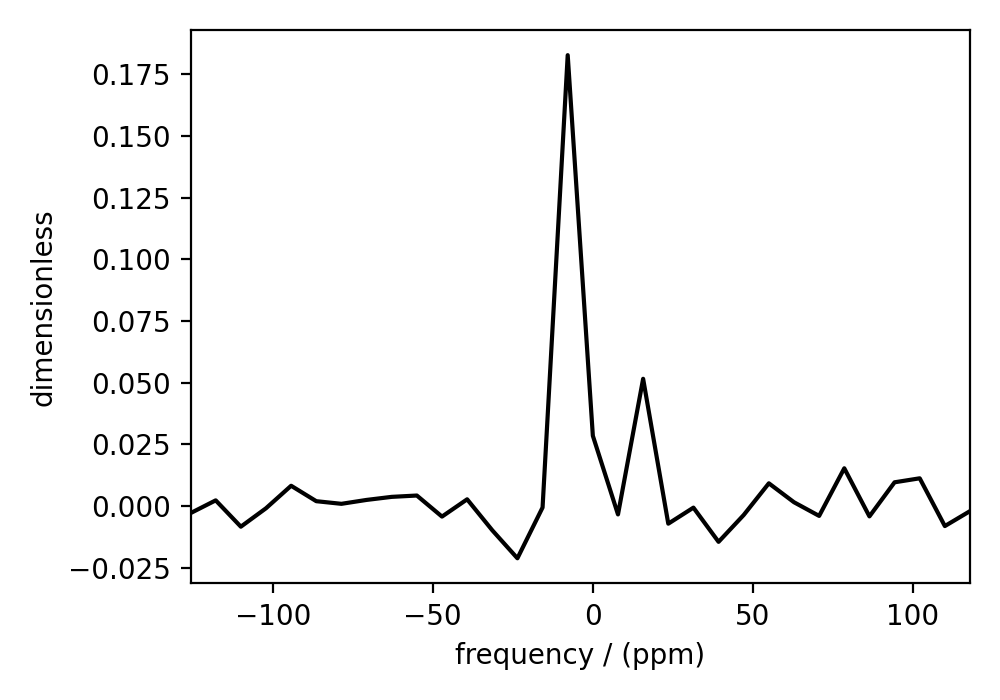
The following is the plot of the spinning sideband spectrum as well as the corresponding true probability distribution.
>>> _, ax = plt.subplots(1, 2, figsize=(9, 3.5), subplot_kw={'projection': 'csdm'})
>>> ax[0].plot(data_object)
>>> ax[0].set_xlabel('frequency / ppm')
>>> ax[0].invert_xaxis()
>>> ax[0].set_title('Pure anisotropic MAS spectrum')
...
>>> plot2D(ax[1], true_data_object, title='True distribution')
>>> plt.tight_layout()
>>> plt.savefig('filename.pdf') # to save figure as editable pdf
>>> plt.show()
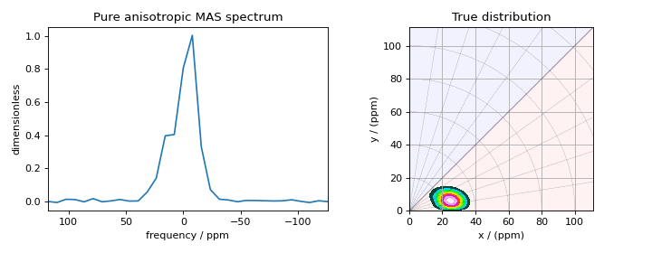

Figure 2 The figure on the left is the pure anisotropic MAS sideband amplitude spectrum corresponding to the nuclear shielding tensor distribution shown on the right.
Dimension Setup
For the inversion, we need to define (1) the coordinates associated with the pure anisotropic dimension, and (2) the two-dimensional x-y coordinates associated with the anisotropic tensor parameters, i.e., the inversion solution grid.
In mrinversion, the anisotropic spectrum dimension is initialized with a
Dimension object from
the csdmpy package. This object holds the
frequency coordinates of the pure anisotropic spectrum. Because the example NMR dataset
is imported as a CSDM object, the anisotropic spectrum dimension is already available as
a CSDM Dimension object in the CSDM object and can be copied from there.
Alternatively, we can create and initialize a anisotropic spectrum dimension using the
csdmpy library as shown below:
>>> anisotropic_dimension = cp.LinearDimension(count=32, increment='625Hz', coordinates_offset='-10kHz')
>>> print(anisotropic_dimension)
LinearDimension([-10000.  -9375.  -8750.  -8125.  -7500.  -6875.  -6250.  -5625.  -5000.
  -4375.  -3750.  -3125.  -2500.  -1875.  -1250.   -625.      0.    625.
   1250.   1875.   2500.   3125.   3750.   4375.   5000.   5625.   6250.
   6875.   7500.   8125.   8750.   9375.] Hz)
Here, the anisotropic dimension is sampled at 625 Hz for 32 points with an offset of -10 kHz.
Similarly, we can create the CSDM dimensions needed for the x-y inversion grid as shown below:
>>> inverse_dimension = [
...     cp.LinearDimension(count=25, increment='370 Hz', label='x'),  # the x-coordinates
...     cp.LinearDimension(count=25, increment='370 Hz', label='y')   # the y-coordinates
... ]
Both dimensions are sampled at every 370 Hz for 25 points. The inverse dimension at index 0 and 1 are the x and y dimensions, respectively.
Generating the kernel
Import the ShieldingPALineshape class and
generate the kernel as follows,
>>> from mrinversion.kernel.nmr import ShieldingPALineshape
>>> lineshapes = ShieldingPALineshape(
...     anisotropic_dimension=anisotropic_dimension,
...     inverse_dimension=inverse_dimension,
...     channel='29Si',
...     magnetic_flux_density='9.4 T',
...     rotor_angle='54.735°',
...     rotor_frequency='625 Hz',
...     number_of_sidebands=32
... )
In the above code, the variable lineshapes is an instance of the
ShieldingPALineshape class. The three required
arguments of this class are the anisotropic_dimension, inverse_dimension, and
channel. We have already defined the first two arguments in the previous subsection.
The value of the channel attribute is the observed nucleus.
The remaining optional arguments are the metadata that describes the environment
under which the spectrum is acquired. In this example, these arguments describe a
\(^{29}\text{Si}\) pure anisotropic spinning-sideband spectrum acquired at 9.4 T
magnetic flux density and spinning at the magic angle (\(54.735^\circ\)) at 625 Hz.
The value of the rotor_frequency argument is the effective anisotropic modulation
frequency. For measurements like PASS 5, the anisotropic modulation frequency is
the physical rotor frequency. For measurements like the extended chemical shift
modulation sequences (XCS) 6, or its variants, where the effective anisotropic
modulation frequency is lower than the physical rotor frequency, then it should be set
accordingly.
The argument number_of_sidebands is the maximum number of sidebands that will be computed per line-shape within the kernel. For most two-dimensional isotropic vs. pure anisotropic spinning-sideband correlation spectra, the sampling along the sideband dimension is the rotor or the effective anisotropic modulation frequency. Therefore, the number_of_sidebands argument is usually the number of points along the sideband dimension. In this example, this value is 32.
Once the ShieldingPALineshape instance is created, use the
kernel() method of the
instance to generate the spinning sideband kernel, as follows,
>>> K = lineshapes.kernel(supersampling=1)
>>> print(K.shape)
(32, 625)
Here, K is the \(32\times 625\) kernel, where the 32 is the number of samples
(sideband amplitudes), and 625 is the number of features (subspectra) on the
\(25 \times 25\) x-y grid. The argument supersampling is the supersampling
factor. In a supersampling scheme, each grid cell is averaged over a \(n\times n\)
sub-grid, where \(n\) is the supersampling factor. A supersampling factor of 1 is
equivalent to no sub-grid averaging.
Data compression (optional)
Often when the kernel, K, is ill-conditioned, the solution becomes unstable in
the presence of the measurement noise. An ill-conditioned kernel is the one
whose singular values quickly decay to zero. In such cases, we employ the
truncated singular value decomposition method to approximately represent the
kernel K onto a smaller sub-space, called the range space, where the
sub-space kernel is relatively well-defined. We refer to this sub-space
kernel as the compressed kernel. Similarly, the measurement data on the
sub-space is referred to as the compressed signal. The compression also
reduces the time for further computation. To compress the kernel and the data,
import the TSVDCompression class and follow,
>>> from mrinversion.linear_model import TSVDCompression
>>> new_system = TSVDCompression(K=K, s=data_object)
compression factor = 1.032258064516129
>>> compressed_K = new_system.compressed_K
>>> compressed_s = new_system.compressed_s
Here, the variable new_system is an instance of the
TSVDCompression class. If no truncation index is
provided as the argument, when initializing the TSVDCompression class, an optimum
truncation index is chosen using the maximum entropy method 7, which is the default
behavior. The attributes compressed_K
and compressed_s holds the
compressed kernel and signal, respectively. The shape of the original signal v.s. the
compressed signal is
>>> print(data_object.shape, compressed_s.shape)
(32,) (31,)
Setting up the inverse problem
When setting up the inversion, we solved the smooth LASSO 8 problem. Read the Smooth-LASSO regularization section for further details.
Import the SmoothLasso class and follow,
>>> from mrinversion.linear_model import SmoothLasso
>>> s_lasso = SmoothLasso(alpha=0.01, lambda1=1e-04, inverse_dimension=inverse_dimension)
Here, the variable s_lasso is an instance of the
SmoothLasso class. The required arguments
of this class are alpha and lambda1, corresponding to the hyperparameters
\(\alpha\) and \(\lambda\), respectively, in the Eq. (5). At the
moment, we don’t know the optimum value of the alpha and lambda1 parameters.
We start with a guess value.
To solve the smooth lasso problem, use the
fit() method of the s_lasso
instance as follows,
>>> s_lasso.fit(K=compressed_K, s=compressed_s)
The two arguments of the fit() method are
the kernel, K, and the signal, s. In the above example, we set the value of K as
compressed_K, and correspondingly the value of s as compressed_s. You may also
use the uncompressed values of the kernel and signal in this method, if desired.
The solution to the smooth lasso is accessed using the
f attribute of the respective object.
>>> f_sol = s_lasso.f
The plot of the solution is
>>> _, ax = plt.subplots(1, 2, figsize=(9, 3.5), subplot_kw={'projection': 'csdm'})
>>> plot2D(ax[0], f_sol/f_sol.max(), title='Guess distribution')
>>> plot2D(ax[1], true_data_object, title='True distribution')
>>> plt.tight_layout()
>>> plt.show()
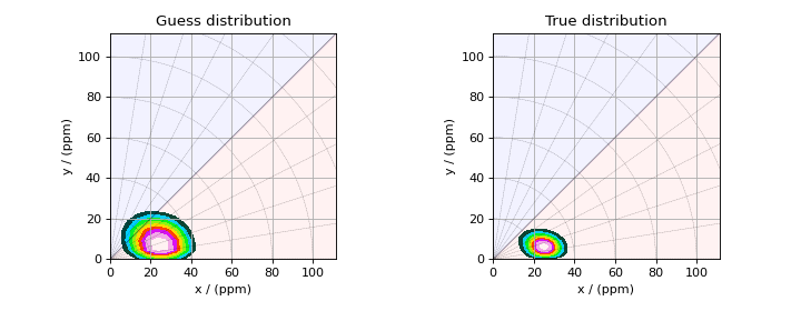
Figure 3 The figure on the left is the guess solution of the nuclear shielding tensor distribution derived from the inversion of the spinning sideband dataset. The figure on the right is the true nuclear shielding tensor distribution.
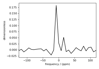
You may also evaluate the residuals corresponding to the solution using the
residuals() method of the object as
follows,
>>> residuals = s_lasso.residuals(K=K, s=data_object)
>>> # the plot of the residuals
>>> plt.figure(figsize=(5, 3.5))
>>> ax = plt.subplot(projection='csdm')
>>> ax.plot(residuals, color='black')
>>> plt.tight_layout()
>>> plt.show()

Figure 4 The residuals between the 1D MAS sideband spectrum and the predicted spectrum from the guess shielding tensor parameter distribution.
The argument of the residuals method is the kernel and the signal data. We provide the original kernel, K, and signal, s, because we desire the residuals corresponding to the original data and not the compressed data.
Statistical learning of tensor parameters
The solution from a linear model trained with the combined l1 and l2 priors, such as the smooth LASSO estimator used here, depends on the choice of the hyperparameters. The solution shown in the above figure is when \(\alpha=0.01\) and \(\lambda=1\times 10^{-4}\). Although it’s a solution, it is unlikely that this is the best solution. For this, we employ the statistical learning-based model, such as the n-fold cross-validation.
The SmoothLassoCV class is designed to solve the
smooth-lasso problem for a range of \(\alpha\) and \(\lambda\) values and
determine the best solution using the n-fold cross-validation. Here, we search the
best model on a \(10 \times 10\) pre-defined \(\alpha\)-\(\lambda\) grid,
using a 10-fold cross-validation statistical learning method. The \(\lambda\) and
\(\alpha\) values are sampled uniformly on a logarithmic scale as,
>>> lambdas = 10 ** (-4 - 2 * (np.arange(10) / 9))
>>> alphas = 10 ** (-3 - 2 * (np.arange(10) / 9))
Smooth-LASSO CV Setup
Setup the smooth lasso cross-validation as follows
>>> from mrinversion.linear_model import SmoothLassoCV
>>> s_lasso_cv = SmoothLassoCV(
...     alphas=alphas,
...     lambdas=lambdas,
...     inverse_dimension=inverse_dimension,
...     sigma=0.005,
...     folds=10
... )
>>> s_lasso_cv.fit(K=compressed_K, s=compressed_s)
The arguments of the SmoothLassoCV is a list
of the alpha and lambda values, along with the standard deviation of the
noise, sigma. The value of the argument folds is the number of folds used in the
cross-validation. As before, to solve the problem, use the
fit() method, whose arguments are
the kernel and signal.
The optimum hyperparameters
The optimized hyperparameters may be accessed using the
hyperparameters attribute of
the class instance,
>>> alpha = s_lasso_cv.hyperparameters['alpha']
>>> lambda_1 = s_lasso_cv.hyperparameters['lambda']
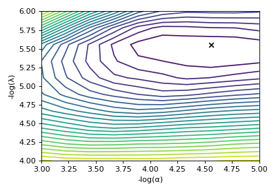
The cross-validation surface
The cross-validation error metric is the mean square error metric. You may access this
data using the cross_validation_curve
attribute.
>>> plt.figure(figsize=(5, 3.5))
>>> ax = plt.subplot(projection='csdm')
>>> ax.contour(np.log10(s_lasso_cv.cross_validation_curve), levels=25)
>>> ax.scatter(-np.log10(s_lasso_cv.hyperparameters['alpha']),
...         -np.log10(s_lasso_cv.hyperparameters['lambda']),
...         marker='x', color='k')
>>> plt.tight_layout()
>>> plt.show()

Figure 5 The ten-folds cross-validation prediction error surface as a function of the hyperparameters \(\alpha\) and \(\beta\).
The optimum solution
The best model selection from the cross-validation method may be accessed using
the f attribute.
>>> f_sol_cv = s_lasso_cv.f # best model selected using the 10-fold cross-validation
The plot of the selected tensor parameter distribution is shown below.
>>> _, ax = plt.subplots(1, 2, figsize=(9, 3.5), subplot_kw={'projection': 'csdm'})
>>> plot2D(ax[0], f_sol_cv/f_sol_cv.max(), title='Optimum distribution')
>>> plot2D(ax[1], true_data_object, title='True distribution')
>>> plt.tight_layout()
>>> plt.show()
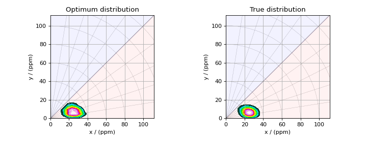
Figure 6 The figure on the left is the optimum solution selected by the 10-folds cross-validation method. The figure on the right is the true model of the nuclear shielding tensor distribution.
See also
- 1
Srivastava, D. J., Vosegaard, T., Massiot, D., Grandinetti, P. J., Core Scientific Dataset Model: A lightweight and portable model and file format for multi-dimensional scientific data. PLOS ONE, 15, 1-38, (2020). DOI:10.1371/journal.pone.0225953
- 2
Bak M., Rasmussen J. T., Nielsen N.C., SIMPSON: A General Simulation Program for Solid-State NMR Spectroscopy. J Magn Reson. 147, 296–330, (2000). DOI:10.1006/jmre.2000.2179
- 3
Massiot D., Fayon F., Capron M., King I., Le Calvé S., Alonso B., et al. Modelling one- and two-dimensional solid-state NMR spectra. Magn Reson Chem. 40, 70–76, (2002) DOI:10.1002/mrc.984
- 4
PhySy Ltd. RMN 2.0; 2019. Available from: https://www.physyapps.com/rmn.
- 5
Dixon, W. T., Spinning sideband free and spinning sideband only NMR spectra in spinning samples. J. Chem. Phys, 77, 1800, (1982). DOI:10.1063/1.444076
- 6
Gullion, T., Extended chemical shift modulation. J. Mag. Res., 85, 3, (1989). DOI:10.1016/0022-2364(89)90253-9
- 7
Varshavsky R., Gottlieb A., Linial M., Horn D., Novel unsupervised feature filtering of biological data. Bioinformatics, 22, e507–e513, (2006). DOI:10.1093/bioinformatics/btl214.
- 8
Hebiri M, Sara A. Van De Geer, The Smooth-Lasso and other l1+l2-penalized methods, arXiv, (2010). arXiv:1003.4885v2