2D MAF data of 2Na2O.3SiO2 glass

The following example illustrates an application of the statistical learning method applied in determining the distribution of the nuclear shielding tensor parameters from a 2D magic-angle flipping (MAF) spectrum. In this example, we use the 2D MAF spectrum 1 of \(2\text{Na}_2\text{O}\cdot3\text{SiO}_2\) glass.

Before getting started

Import all relevant packages.

import csdmpy as cp
import matplotlib.pyplot as plt
import numpy as np
from matplotlib import cm

from mrinversion.kernel.nmr import ShieldingPALineshape
from mrinversion.linear_model import SmoothLasso, TSVDCompression
from mrinversion.utils import plot_3d, to_Haeberlen_grid

Setup for the matplotlib figures.

def plot2D(csdm_object, **kwargs):
    plt.figure(figsize=(4.5, 3.5))
    ax = plt.subplot(projection="csdm")
    ax.imshow(csdm_object, cmap="gist_ncar_r", aspect="auto", **kwargs)
    ax.invert_xaxis()
    ax.invert_yaxis()
    plt.tight_layout()
    plt.show()

Dataset setup

Import the dataset

Load the dataset. Here, we import the dataset as the CSDM data-object.

# The 2D MAF dataset in csdm format
filename = "https://osu.box.com/shared/static/k405dsptwe1p43x8mfi1wc1geywrypzc.csdf"
data_object = cp.load(filename)

# For inversion, we only interest ourselves with the real part of the complex dataset.
data_object = data_object.real

# We will also convert the coordinates of both dimensions from Hz to ppm.
_ = [item.to("ppm", "nmr_frequency_ratio") for item in data_object.dimensions]

Here, the variable data_object is a CSDM object that holds the real part of the 2D MAF dataset. The plot of the 2D MAF dataset is

plot2D(data_object)

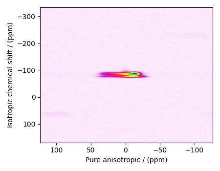
There are two dimensions in this dataset. The dimension at index 0 is the pure anisotropic dimension, while the dimension at index 1 is the isotropic chemical shift dimension.

Prepping the data for inversion

Step-1: Data Alignment

When using the csdm objects with the mrinversion package, the dimension at index 0 must be the dimension undergoing the linear inversion. In this example, we plan to invert the pure anisotropic shielding line-shape. In the data_object, the anisotropic dimension is already at index 0 and, therefore, no further action is required.

Step-2: Optimization

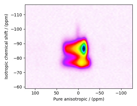
Also notice, the signal from the 2D MAF dataset occupies a small fraction of the two-dimensional frequency grid. For optimum performance, truncate the dataset to the relevant region before proceeding. Use the appropriate array indexing/slicing to select the signal region.

data_object_truncated = data_object[:, 220:280]
plot2D(data_object_truncated)

Linear Inversion setup

Dimension setup

Anisotropic-dimension: The dimension of the dataset that holds the pure anisotropic frequency contributions. In mrinversion, this must always be the dimension at index 0 of the data object.

anisotropic_dimension = data_object_truncated.dimensions[0]

x-y dimensions: The two inverse dimensions corresponding to the x and y-axis of the x-y grid.

inverse_dimensions = [
    cp.LinearDimension(count=25, increment="500 Hz", label="x"),  # the `x`-dimension.
    cp.LinearDimension(count=25, increment="500 Hz", label="y"),  # the `y`-dimension.
]

Generating the kernel

For MAF datasets, the line-shape kernel corresponds to the pure nuclear shielding anisotropy line-shapes. Use the ShieldingPALineshape class to generate a shielding line-shape kernel.

lineshape = ShieldingPALineshape(
    anisotropic_dimension=anisotropic_dimension,
    inverse_dimension=inverse_dimensions,
    channel="29Si",
    magnetic_flux_density="9.4 T",
    rotor_angle="90°",
    rotor_frequency="12 kHz",
    number_of_sidebands=4,
)

Here, lineshape is an instance of the ShieldingPALineshape class. The required arguments of this class are the anisotropic_dimension, inverse_dimension, and channel. We have already defined the first two arguments in the previous sub-section. The value of the channel argument is the nucleus observed in the MAF experiment. In this example, this value is ‘29Si’. The remaining arguments, such as the magnetic_flux_density, rotor_angle, and rotor_frequency, are set to match the conditions under which the 2D MAF spectrum was acquired. The value of the number_of_sidebands argument is the number of sidebands calculated for each line-shape within the kernel. Unless, you have a lot of spinning sidebands in your MAF dataset, four sidebands should be enough.

Once the ShieldingPALineshape instance is created, use the kernel() method of the instance to generate the MAF line-shape kernel.

K = lineshape.kernel(supersampling=1)
print(K.shape)

Out:

(128, 625)

The kernel K is a NumPy array of shape (128, 625), where the axes with 128 and 625 points are the anisotropic dimension and the features (x-y coordinates) corresponding to the \(25\times 25\) x-y grid, respectively.

Data Compression

Data compression is optional but recommended. It may reduce the size of the inverse problem and, thus, further computation time.

new_system = TSVDCompression(K, data_object_truncated)
compressed_K = new_system.compressed_K
compressed_s = new_system.compressed_s

print(f"truncation_index = {new_system.truncation_index}")

Out:

compression factor = 1.1851851851851851
truncation_index = 108

Solving the inverse problem

Smooth LASSO cross-validation

Solve the smooth-lasso problem. Ordinarily, one should use the statistical learning method to solve the inverse problem over a range of α and λ values and then determine the best nuclear shielding tensor parameter distribution for the given 2D MAF dataset. Considering the limited build time for the documentation, we skip this step and evaluate the distribution at pre-optimized α and λ values. The optimum values are \(\alpha = 2.2\times 10^{-8}\) and \(\lambda = 1.27\times 10^{-6}\). The following commented code was used in determining the optimum α and λ values.

# from mrinversion.linear_model import SmoothLassoCV
# import numpy as np

# # setup the pre-defined range of alpha and lambda values
# lambdas = 10 ** (-4 - 3 * (np.arange(20) / 19))
# alphas = 10 ** (-4.5 - 5 * (np.arange(20) / 19))

# # setup the smooth lasso cross-validation class
# s_lasso = SmoothLassoCV(
#     alphas=alphas,  # A numpy array of alpha values.
#     lambdas=lambdas,  # A numpy array of lambda values.
#     sigma=0.003,  # The standard deviation of noise from the MAF data.
#     folds=10,  # The number of folds in n-folds cross-validation.
#     inverse_dimension=inverse_dimensions,  # previously defined inverse dimensions.
#     verbose=1,  # If non-zero, prints the progress as the computation proceeds.
# )

# # run fit using the compressed kernel and compressed data.
# s_lasso.fit(compressed_K, compressed_s)

# # the optimum hyper-parameters, alpha and lambda, from the cross-validation.
# print(s_lasso.hyperparameters)
# # {'alpha': 2.198392648862289e-08, 'lambda': 1.2742749857031348e-06}

# # the solution
# f_sol = s_lasso.f

# # the cross-validation error curve
# CV_metric = s_lasso.cross_validation_curve

If you use the above SmoothLassoCV method, skip the following code-block.

# Setup the smooth lasso class
s_lasso = SmoothLasso(
    alpha=2.198e-8, lambda1=1.27e-6, inverse_dimension=inverse_dimensions
)
# run the fit method on the compressed kernel and compressed data.
s_lasso.fit(K=compressed_K, s=compressed_s)

The optimum solution

The f attribute of the instance holds the solution,

f_sol = s_lasso.f  # f_sol is a CSDM object.

where f_sol is the optimum solution.

The fit residuals

To calculate the residuals between the data and predicted data(fit), use the residuals() method, as follows,

residuals = s_lasso.residuals(K=K, s=data_object_truncated)
# residuals is a CSDM object.

# The plot of the residuals.
plot2D(residuals, vmax=data_object_truncated.max(), vmin=data_object_truncated.min())

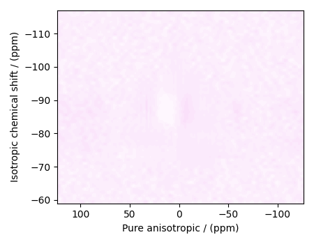
The standard deviation of the residuals is

residuals.std()

Out:

<Quantity 0.00347761>

Saving the solution

To serialize the solution to a file, use the save() method of the CSDM object, for example,

f_sol.save("2Na2O.3SiO2_inverse.csdf")  # save the solution
residuals.save("2Na2O.3SiO2_residue.csdf")  # save the residuals

Data Visualization

At this point, we have solved the inverse problem and obtained an optimum distribution of the nuclear shielding tensor parameters from the 2D MAF dataset. You may use any data visualization and interpretation tool of choice for further analysis. In the following sections, we provide minimal visualization to complete the case study.

Visualizing the 3D solution

# Normalize the solution
f_sol /= f_sol.max()

# Convert the coordinates of the solution, `f_sol`, from Hz to ppm.
[item.to("ppm", "nmr_frequency_ratio") for item in f_sol.dimensions]

# The 3D plot of the solution
plt.figure(figsize=(5, 4.4))
ax = plt.subplot(projection="3d")
plot_3d(ax, f_sol, elev=25, azim=-50, x_lim=[0, 150], y_lim=[0, 150], z_lim=[-60, -120])
plt.tight_layout()
plt.show()

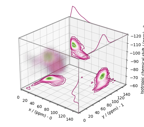
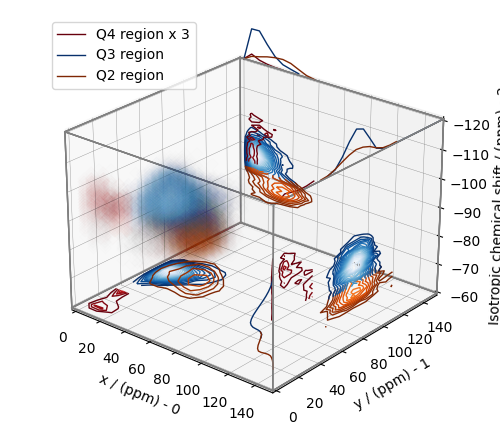
From the 3D plot, we observe three distinct regions corresponding to the \(\text{Q}^4\), \(\text{Q}^3\), and \(\text{Q}^2\) sites, respectively. The \(\text{Q}^4\) sites are resolved in the 3D distribution; however, we observe partial overlapping \(\text{Q}^3\) and \(\text{Q}^2\) sites. The following is a naive selection of the three regions. One may also apply sophisticated classification algorithms to better quantify the Q-species.

Q4_region = f_sol[0:6, 0:6, 14:35] * 3
Q4_region.description = "Q4 region x 3"

Q3_region = f_sol[0:8, 7:, 20:39]
Q3_region.description = "Q3 region"

Q2_region = f_sol[:10, 6:18, 36:52]
Q2_region.description = "Q2 region"

An approximate plot of the respective regions is shown below.

# Calculate the normalization factor for the 2D contours and 1D projections from the
# original solution, `f_sol`. Use this normalization factor to scale the intensities
# from the sub-regions.
max_2d = [
    f_sol.sum(axis=0).max().value,
    f_sol.sum(axis=1).max().value,
    f_sol.sum(axis=2).max().value,
]
max_1d = [
    f_sol.sum(axis=(1, 2)).max().value,
    f_sol.sum(axis=(0, 2)).max().value,
    f_sol.sum(axis=(0, 1)).max().value,
]

plt.figure(figsize=(5, 4.4))
ax = plt.subplot(projection="3d")

# plot for the Q4 region
plot_3d(
    ax,
    Q4_region,
    x_lim=[0, 150],  # the x-limit
    y_lim=[0, 150],  # the y-limit
    z_lim=[-60, -120],  # the z-limit
    max_2d=max_2d,  # normalization factors for the 2D contours projections
    max_1d=max_1d,  # normalization factors for the 1D projections
    cmap=cm.Reds_r,  # colormap
)
# plot for the Q3 region
plot_3d(
    ax,
    Q3_region,
    x_lim=[0, 150],  # the x-limit
    y_lim=[0, 150],  # the y-limit
    z_lim=[-60, -120],  # the z-limit
    max_2d=max_2d,  # normalization factors for the 2D contours projections
    max_1d=max_1d,  # normalization factors for the 1D projections
    cmap=cm.Blues_r,  # colormap
)
# plot for the Q2 region
plot_3d(
    ax,
    Q2_region,
    elev=25,  # the elevation angle in the z plane
    azim=-50,  # the azimuth angle in the x-y plane
    x_lim=[0, 150],  # the x-limit
    y_lim=[0, 150],  # the y-limit
    z_lim=[-60, -120],  # the z-limit
    max_2d=max_2d,  # normalization factors for the 2D contours projections
    max_1d=max_1d,  # normalization factors for the 1D projections
    cmap=cm.Oranges_r,  # colormap
    box=False,  # draw a box around the region
)
ax.legend()
plt.tight_layout()
plt.show()

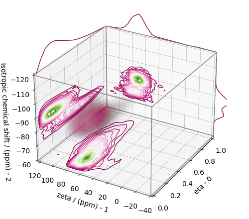
Convert the 3D tensor distribution in Haeberlen parameters

You may re-bin the 3D tensor parameter distribution from a \(\rho(\delta_\text{iso}, x, y)\) distribution to \(\rho(\delta_\text{iso}, \zeta_\sigma, \eta_\sigma)\) distribution as follows.

# Create the zeta and eta dimensions,, as shown below.
zeta = cp.as_dimension(np.arange(40) * 4 - 40, unit="ppm", label="zeta")
eta = cp.as_dimension(np.arange(16) / 15, label="eta")

# Use the `to_Haeberlen_grid` function to convert the tensor parameter distribution.
fsol_Hae = to_Haeberlen_grid(f_sol, zeta, eta)

The 3D plot

plt.figure(figsize=(5, 4.4))
ax = plt.subplot(projection="3d")
plot_3d(ax, fsol_Hae, x_lim=[0, 1], y_lim=[-40, 120], z_lim=[-60, -120], alpha=0.1)
plt.tight_layout()
plt.show()

References

1

Zhang, P., Dunlap, C., Florian, P., Grandinetti, P. J., Farnan, I., Stebbins , J. F. Silicon site distributions in an alkali silicate glass derived by two-dimensional 29Si nuclear magnetic resonance, J. Non. Cryst. Solids, 204, (1996), 294–300. doi:10.1016/S0022-3093(96)00601-1.