2D MAF data of Rb2O.2.25SiO2 glass

The following example is an application of the statistical learning method in determining the distribution of the nuclear shielding tensor parameters from a 2D magic-angle flipping (MAF) spectrum. In this example, we use the 2D MAF spectrum 1 of \(\text{Rb}_2\text{O}\cdot2.25\text{SiO}_2\) glass.

Before getting started

Import all relevant packages.

import csdmpy as cp
import matplotlib.pyplot as plt
import numpy as np
from matplotlib import cm
from csdmpy import statistics as stats

from mrinversion.kernel.nmr import ShieldingPALineshape
from mrinversion.kernel.utils import x_y_to_zeta_eta
from mrinversion.linear_model import SmoothLassoCV, TSVDCompression
from mrinversion.utils import plot_3d, to_Haeberlen_grid

Setup for the matplotlib figures.

# function for plotting 2D dataset
def plot2D(csdm_object, **kwargs):
    plt.figure(figsize=(4.5, 3.5))
    ax = plt.subplot(projection="csdm")
    ax.imshow(csdm_object, cmap="gist_ncar_r", aspect="auto", **kwargs)
    ax.invert_xaxis()
    ax.invert_yaxis()
    plt.tight_layout()
    plt.show()

Dataset setup

Import the dataset

Load the dataset. In this example, we import the dataset as the CSDM data-object.

# The 2D MAF dataset in csdm format
filename = "https://zenodo.org/record/3964531/files/Rb2O-2_25SiO2-MAF.csdf"
data_object = cp.load(filename)

# For inversion, we only interest ourselves with the real part of the complex dataset.
data_object = data_object.real

# We will also convert the coordinates of both dimensions from Hz to ppm.
_ = [item.to("ppm", "nmr_frequency_ratio") for item in data_object.dimensions]

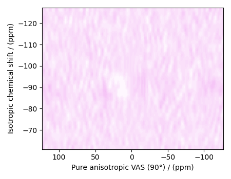
Here, the variable data_object is a CSDM object that holds the real part of the 2D MAF dataset. The plot of the 2D MAF dataset is

plot2D(data_object)

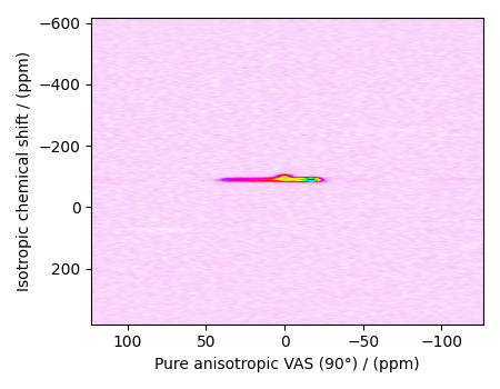
There are two dimensions in this dataset. The dimension at index 0, the horizontal dimension in the figure, is the pure anisotropic dimension, while the dimension at index 1, the vertical dimension, is the isotropic chemical shift dimension. The number of coordinates along the respective dimensions is

print(data_object.shape)

Out:

(128, 512)

with 128 points along the anisotropic dimension (index 0) and 512 points along the isotropic chemical shift dimension (index 1).

Prepping the data for inversion

Step-1: Data Alignment

When using the csdm objects with the mrinversion package, the dimension at index 0 must be the dimension undergoing the linear inversion. In this example, we plan to invert the pure anisotropic shielding line-shape. Since the anisotropic dimension in data_object is already at index 0, no further action is required.

Step-2: Optimization

Notice, the signal from the 2D MAF dataset occupies a small fraction of the two-dimensional frequency grid. Though you may choose to proceed with the inversion directly onto this dataset, it is not computationally optimum. For optimum performance, trim the dataset to the region of relevant signals. Use the appropriate array indexing/slicing to select the signal region.

data_object_truncated = data_object[:, 250:285]
plot2D(data_object_truncated)

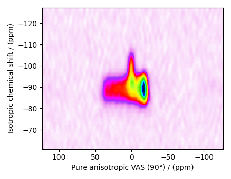
In the above code, we truncate the isotropic chemical shifts, dimension at index 1, to coordinate between indexes 250 and 285. The isotropic shift coordinates from the truncated dataset are

print(data_object_truncated.dimensions[1].coordinates)

Out:

[-127.27782256 -125.3275251  -123.37722764 -121.42693019 -119.47663273
 -117.52633527 -115.57603781 -113.62574035 -111.6754429  -109.72514544
 -107.77484798 -105.82455052 -103.87425306 -101.92395561  -99.97365815
  -98.02336069  -96.07306323  -94.12276577  -92.17246832  -90.22217086
  -88.2718734   -86.32157594  -84.37127848  -82.42098103  -80.47068357
  -78.52038611  -76.57008865  -74.6197912   -72.66949374  -70.71919628
  -68.76889882  -66.81860136  -64.86830391  -62.91800645  -60.96770899] ppm

Linear Inversion setup

Dimension setup

In a generic linear-inverse problem, one needs to define two sets of dimensions—the dimensions undergoing a linear transformation, and the dimensions onto which the inversion method transforms the data. In the line-shape inversion, the two sets of dimensions are the anisotropic dimension and the x-y dimensions.

Anisotropic-dimension: The dimension of the dataset that holds the pure anisotropic frequency contributions. In mrinversion, this must always be the dimension at index 0 of the data object.

anisotropic_dimension = data_object_truncated.dimensions[0]

x-y dimensions: The two inverse dimensions corresponding to the x and y-axis of the x-y grid.

inverse_dimensions = [
    cp.LinearDimension(count=25, increment="400 Hz", label="x"),  # the `x`-dimension.
    cp.LinearDimension(count=25, increment="400 Hz", label="y"),  # the `y`-dimension.
]

Generating the kernel

For MAF datasets, the line-shape kernel corresponds to the pure nuclear shielding anisotropy line-shapes. Use the ShieldingPALineshape class to generate a shielding line-shape kernel.

lineshape = ShieldingPALineshape(
    anisotropic_dimension=anisotropic_dimension,
    inverse_dimension=inverse_dimensions,
    channel="29Si",
    magnetic_flux_density="9.4 T",
    rotor_angle="90°",
    rotor_frequency="13 kHz",
    number_of_sidebands=4,
)

Here, lineshape is an instance of the ShieldingPALineshape class. The required arguments of this class are the anisotropic_dimension, inverse_dimension, and channel. We have already defined the first two arguments in the previous sub-section. The value of the channel argument is the nucleus observed in the MAF experiment. In this example, this value is ‘29Si’. The remaining arguments, such as the magnetic_flux_density, rotor_angle, and rotor_frequency, are set to match the conditions under which the 2D MAF spectrum was acquired. Note for the MAF measurements the rotor angle is usually \(90^\circ\) for the anisotropic dimension. The value of the number_of_sidebands argument is the number of sidebands calculated for each line-shape within the kernel. Unless, you have a lot of spinning sidebands in your MAF dataset, the value of this argument is generally low. Here, we calculate four spinning sidebands per line-shape within in the kernel.

Once the ShieldingPALineshape instance is created, use the kernel() method of the instance to generate the MAF line-shape kernel.

K = lineshape.kernel(supersampling=1)
print(K.shape)

Out:

(128, 625)

The kernel K is a NumPy array of shape (128, 625), where the axes with 128 and 625 points are the anisotropic dimension and the features (x-y coordinates) corresponding to the \(25\times 25\) x-y grid, respectively.

Data Compression

Data compression is optional but recommended. It may reduce the size of the inverse problem and, thus, further computation time.

new_system = TSVDCompression(K, data_object_truncated)
compressed_K = new_system.compressed_K
compressed_s = new_system.compressed_s

print(f"truncation_index = {new_system.truncation_index}")

Out:

compression factor = 1.471264367816092
truncation_index = 87

Solving the inverse problem

Smooth LASSO cross-validation

Solve the smooth-lasso problem. Use the statistical learning SmoothLassoCV method to solve the inverse problem over a range of α and λ values and determine the best nuclear shielding tensor parameter distribution for the given 2D MAF dataset. Considering the limited build time for the documentation, we’ll perform the cross-validation over a smaller \(5 \times 5\) x-y grid. You may increase the grid resolution for your problem if desired.

# setup the pre-defined range of alpha and lambda values
lambdas = 10 ** (-5.2 - 1.25 * (np.arange(5) / 4))
alphas = 10 ** (-5.5 - 1.25 * (np.arange(5) / 4))

# setup the smooth lasso cross-validation class
s_lasso = SmoothLassoCV(
    alphas=alphas,  # A numpy array of alpha values.
    lambdas=lambdas,  # A numpy array of lambda values.
    sigma=0.0045,  # The standard deviation of noise from the 2D MAF data.
    folds=10,  # The number of folds in n-folds cross-validation.
    inverse_dimension=inverse_dimensions,  # previously defined inverse dimensions.
    verbose=1,  # If non-zero, prints the progress as the computation proceeds.
)

# run the fit method on the compressed kernel and compressed data.
s_lasso.fit(K=compressed_K, s=compressed_s)

Out:

[Parallel(n_jobs=-1)]: Using backend ThreadingBackend with 2 concurrent workers.
[Parallel(n_jobs=-1)]: Done   5 out of   5 | elapsed:    6.8s finished
[Parallel(n_jobs=-1)]: Using backend ThreadingBackend with 2 concurrent workers.
[Parallel(n_jobs=-1)]: Done   5 out of   5 | elapsed:    7.3s finished
[Parallel(n_jobs=-1)]: Using backend ThreadingBackend with 2 concurrent workers.
[Parallel(n_jobs=-1)]: Done   5 out of   5 | elapsed:    8.2s finished
[Parallel(n_jobs=-1)]: Using backend ThreadingBackend with 2 concurrent workers.
[Parallel(n_jobs=-1)]: Done   5 out of   5 | elapsed:    9.6s finished
[Parallel(n_jobs=-1)]: Using backend ThreadingBackend with 2 concurrent workers.
[Parallel(n_jobs=-1)]: Done   5 out of   5 | elapsed:   11.7s finished

The optimum hyper-parameters

Use the hyperparameters attribute of the instance for the optimum hyper-parameters, \(\alpha\) and \(\lambda\), determined from the cross-validation.

print(s_lasso.hyperparameters)

Out:

{'alpha': 7.498942093324558e-07, 'lambda': 3.0725573652674454e-06}

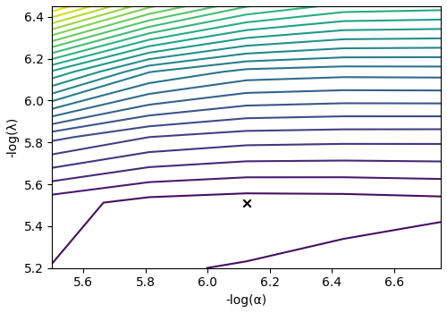
The cross-validation surface

Optionally, you may want to visualize the cross-validation error curve/surface. Use the cross_validation_curve attribute of the instance, as follows

CV_metric = s_lasso.cross_validation_curve  # `CV_metric` is a CSDM object.

# plot of the cross validation surface
plt.figure(figsize=(5, 3.5))
ax = plt.subplot(projection="csdm")
ax.contour(np.log10(CV_metric), levels=25)
ax.scatter(
    -np.log10(s_lasso.hyperparameters["alpha"]),
    -np.log10(s_lasso.hyperparameters["lambda"]),
    marker="x",
    color="k",
)
plt.tight_layout(pad=0.5)
plt.show()

The optimum solution

The f attribute of the instance holds the solution corresponding to the optimum hyper-parameters,

f_sol = s_lasso.f  # f_sol is a CSDM object.

where f_sol is the optimum solution.

The fit residuals

To calculate the residuals between the data and predicted data(fit), use the residuals() method, as follows,

residuals = s_lasso.residuals(K=K, s=data_object_truncated)
# residuals is a CSDM object.

# The plot of the residuals.
plot2D(residuals, vmax=data_object_truncated.max(), vmin=data_object_truncated.min())

The standard deviation of the residuals is close to the standard deviation of the noise, \(\sigma = 0.0043\).

residuals.std()

Out:

<Quantity 0.00475719>

Saving the solution

To serialize the solution (nuclear shielding tensor parameter distribution) to a file, use the save() method of the CSDM object, for example,

f_sol.save("Rb2O.2.25SiO2_inverse.csdf")  # save the solution
residuals.save("Rb2O.2.25SiO2_residue.csdf")  # save the residuals

Data Visualization

At this point, we have solved the inverse problem and obtained an optimum distribution of the nuclear shielding tensor parameters from the 2D MAF dataset. You may use any data visualization and interpretation tool of choice for further analysis. In the following sections, we provide minimal visualization and analysis to complete the case study.

Visualizing the 3D solution

# Normalize the solution
f_sol /= f_sol.max()

# Convert the coordinates of the solution, `f_sol`, from Hz to ppm.
[item.to("ppm", "nmr_frequency_ratio") for item in f_sol.dimensions]

# The 3D plot of the solution
plt.figure(figsize=(5, 4.4))
ax = plt.subplot(projection="3d")
plot_3d(ax, f_sol, x_lim=[0, 150], y_lim=[0, 150], z_lim=[-50, -150])
plt.tight_layout()
plt.show()

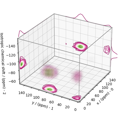
From the 3D plot, we observe two distinct regions: one for the \(\text{Q}^4\) sites and another for the \(\text{Q}^3\) sites. Select the respective regions by using the appropriate array indexing,

Q4_region = f_sol[0:7, 0:7, 4:25]
Q4_region.description = "Q4 region"

Q3_region = f_sol[0:8, 10:24, 11:30]
Q3_region.description = "Q3 region"

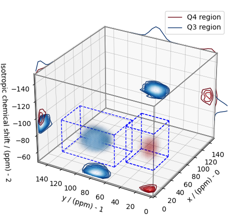
The plot of the respective regions is shown below.

# Calculate the normalization factor for the 2D contours and 1D projections from the
# original solution, `f_sol`. Use this normalization factor to scale the intensities
# from the sub-regions.
max_2d = [
    f_sol.sum(axis=0).max().value,
    f_sol.sum(axis=1).max().value,
    f_sol.sum(axis=2).max().value,
]
max_1d = [
    f_sol.sum(axis=(1, 2)).max().value,
    f_sol.sum(axis=(0, 2)).max().value,
    f_sol.sum(axis=(0, 1)).max().value,
]

plt.figure(figsize=(5, 4.4))
ax = plt.subplot(projection="3d")

# plot for the Q4 region
plot_3d(
    ax,
    Q4_region,
    x_lim=[0, 150],  # the x-limit
    y_lim=[0, 150],  # the y-limit
    z_lim=[-50, -150],  # the z-limit
    max_2d=max_2d,  # normalization factors for the 2D contours projections
    max_1d=max_1d,  # normalization factors for the 1D projections
    cmap=cm.Reds_r,  # colormap
    box=True,  # draw a box around the region
)
# plot for the Q3 region
plot_3d(
    ax,
    Q3_region,
    x_lim=[0, 150],  # the x-limit
    y_lim=[0, 150],  # the y-limit
    z_lim=[-50, -150],  # the z-limit
    max_2d=max_2d,  # normalization factors for the 2D contours projections
    max_1d=max_1d,  # normalization factors for the 1D projections
    cmap=cm.Blues_r,  # colormap
    box=True,  # draw a box around the region
)
ax.legend()
plt.tight_layout()
plt.show()

Visualizing the isotropic projections.

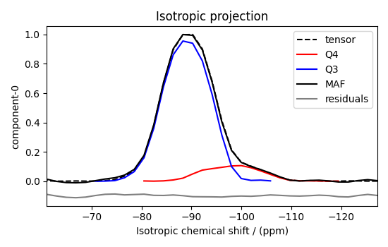
Because the \(\text{Q}^4\) and \(\text{Q}^3\) regions are fully resolved after the inversion, evaluating the contributions from these regions is trivial. For examples, the distribution of the isotropic chemical shifts for these regions are

# Isotropic chemical shift projection of the 2D MAF dataset.
data_iso = data_object_truncated.sum(axis=0)
data_iso /= data_iso.max()  # normalize the projection

# Isotropic chemical shift projection of the tensor distribution dataset.
f_sol_iso = f_sol.sum(axis=(0, 1))

# Isotropic chemical shift projection of the tensor distribution for the Q4 region.
Q4_region_iso = Q4_region.sum(axis=(0, 1))

# Isotropic chemical shift projection of the tensor distribution for the Q3 region.
Q3_region_iso = Q3_region.sum(axis=(0, 1))

# Normalize the three projections.
f_sol_iso_max = f_sol_iso.max()
f_sol_iso /= f_sol_iso_max
Q4_region_iso /= f_sol_iso_max
Q3_region_iso /= f_sol_iso_max

# The plot of the different projections.
plt.figure(figsize=(5.5, 3.5))
ax = plt.subplot(projection="csdm")
ax.plot(f_sol_iso, "--k", label="tensor")
ax.plot(Q4_region_iso, "r", label="Q4")
ax.plot(Q3_region_iso, "b", label="Q3")
ax.plot(data_iso, "-k", label="MAF")
ax.plot(data_iso - f_sol_iso - 0.1, "gray", label="residuals")
ax.set_title("Isotropic projection")
ax.invert_xaxis()
plt.legend()
plt.tight_layout()
plt.show()

Analysis

For the analysis, we use the statistics module of the csdmpy package. Following is the moment analysis of the 3D volumes for both the \(\text{Q}^4\) and \(\text{Q}^3\) regions up to the second moment.

int_Q4 = stats.integral(Q4_region)  # volume of the Q4 distribution
mean_Q4 = stats.mean(Q4_region)  # mean of the Q4 distribution
std_Q4 = stats.std(Q4_region)  # standard deviation of the Q4 distribution

int_Q3 = stats.integral(Q3_region)  # volume of the Q3 distribution
mean_Q3 = stats.mean(Q3_region)  # mean of the Q3 distribution
std_Q3 = stats.std(Q3_region)  # standard deviation of the Q3 distribution

print("Q4 statistics")
print(f"\tpopulation = {100 * int_Q4 / (int_Q4 + int_Q3)}%")
print("\tmean\n\t\tx:\t{0}\n\t\ty:\t{1}\n\t\tiso:\t{2}".format(*mean_Q4))
print("\tstandard deviation\n\t\tx:\t{0}\n\t\ty:\t{1}\n\t\tiso:\t{2}".format(*std_Q4))

print("Q3 statistics")
print(f"\tpopulation = {100 * int_Q3 / (int_Q4 + int_Q3)}%")
print("\tmean\n\t\tx:\t{0}\n\t\ty:\t{1}\n\t\tiso:\t{2}".format(*mean_Q3))
print("\tstandard deviation\n\t\tx:\t{0}\n\t\ty:\t{1}\n\t\tiso:\t{2}".format(*std_Q3))

Out:

Q4 statistics
        population = 11.890539677377667%
        mean
                x:      8.278439388848904 ppm
                y:      8.720854288316803 ppm
                iso:    -98.05908068021311 ppm
        standard deviation
                x:      4.367435149315327 ppm
                y:      4.694619674817486 ppm
                iso:    5.396280313955067 ppm
Q3 statistics
        population = 88.10946032262234%
        mean
                x:      10.130212774789943 ppm
                y:      79.93509495728581 ppm
                iso:    -88.92549894517143 ppm
        standard deviation
                x:      6.6364608363215 ppm
                y:      8.121016875697714 ppm
                iso:    4.40509781257238 ppm

The statistics shown above are according to the respective dimensions, that is, the x, y, and the isotropic chemical shifts. To convert the x and y statistics to commonly used \(\zeta_\sigma\) and \(\eta_\sigma\) statistics, use the x_y_to_zeta_eta() function.

mean_ζη_Q3 = x_y_to_zeta_eta(*mean_Q3[0:2])

# error propagation for calculating the standard deviation
std_ζ = (std_Q3[0] * mean_Q3[0]) ** 2 + (std_Q3[1] * mean_Q3[1]) ** 2
std_ζ /= mean_Q3[0] ** 2 + mean_Q3[1] ** 2
std_ζ = np.sqrt(std_ζ)

std_η = (std_Q3[1] * mean_Q3[0]) ** 2 + (std_Q3[0] * mean_Q3[1]) ** 2
std_η /= (mean_Q3[0] ** 2 + mean_Q3[1] ** 2) ** 2
std_η = (4 / np.pi) * np.sqrt(std_η)

print("Q3 statistics")
print(f"\tpopulation = {100 * int_Q3 / (int_Q4 + int_Q3)}%")
print("\tmean\n\t\tζ:\t{0}\n\t\tη:\t{1}\n\t\tiso:\t{2}".format(*mean_ζη_Q3, mean_Q3[2]))
print(
    "\tstandard deviation\n\t\tζ:\t{0}\n\t\tη:\t{1}\n\t\tiso:\t{2}".format(
        std_ζ, std_η, std_Q3[2]
    )
)

Out:

Q3 statistics
        population = 88.10946032262234%
        mean
                ζ:      80.57444146063203 ppm
                η:      0.16050264820969595
                iso:    -88.92549894517143 ppm
        standard deviation
                ζ:      8.099667652306346 ppm
                η:      0.10528101479643995
                iso:    4.40509781257238 ppm

Result cross-verification

The reported value for the Qn-species distribution from Baltisberger et. al. 1 is listed below and is consistent with the above result.

Species	Yield	Isotropic chemical shift, \(\delta_\text{iso}\)	Shielding anisotropy, \(\zeta_\sigma\):	Shielding asymmetry, \(\eta_\sigma\):
Q4	\(11.0 \pm 0.3\) %	\(-98.0 \pm 5.64\) ppm	0 ppm (fixed)	0 (fixed)
Q3	\(89 \pm 0.1\) %	\(-89.5 \pm 4.65\) ppm	80.7 ppm with a 6.7 ppm Gaussian broadening	0 (fixed)

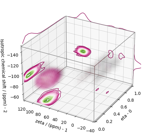
Convert the 3D tensor distribution in Haeberlen parameters

You may re-bin the 3D tensor parameter distribution from a \(\rho(\delta_\text{iso}, x, y)\) distribution to \(\rho(\delta_\text{iso}, \zeta_\sigma, \eta_\sigma)\) distribution as follows.

# Create the zeta and eta dimensions,, as shown below.
zeta = cp.as_dimension(np.arange(40) * 4 - 40, unit="ppm", label="zeta")
eta = cp.as_dimension(np.arange(16) / 15, label="eta")

# Use the `to_Haeberlen_grid` function to convert the tensor parameter distribution.
fsol_Hae = to_Haeberlen_grid(f_sol, zeta, eta)

The 3D plot

plt.figure(figsize=(5, 4.4))
ax = plt.subplot(projection="3d")
plot_3d(ax, fsol_Hae, x_lim=[0, 1], y_lim=[-40, 120], z_lim=[-50, -150], alpha=0.4)
plt.tight_layout()
plt.show()

References

1(1,2)

Baltisberger, J. H., Florian, P., Keeler, E. G., Phyo, P. A., Sanders, K. J., Grandinetti, P. J.. Modifier cation effects on 29Si nuclear shielding anisotropies in silicate glasses, J. Magn. Reson. 268 (2016) 95 – 106. doi:10.1016/j.jmr.2016.05.003.