Utils
- mrinversion.kernel.utils.x_y_to_zeta_eta(x, y)[source]
Convert the coordinates \((x,y)\) to \((\zeta, \eta)\) using the following definition,
(24)¶\[\begin{split}\left.\begin{array}{rl} \zeta &= \sqrt{x^2 + y^2}, \\ \eta &= \frac{4}{\pi} \tan^{-1} \left| \frac{x}{y} \right| \end{array} {~~~~~~~~} \right\} {~~~~~~~~} |x| \le |y|.\end{split}\](25)¶\[\begin{split}\left.\begin{array}{rl} \zeta &= -\sqrt{x^2 + y^2}, \\ \eta &= \frac{4}{\pi} \tan^{-1} \left| \frac{y}{x} \right| \end{array} {~~~~~~~~} \right\} {~~~~~~~~} |x| > |y|.\end{split}\]- Parameters:
x – floats or Quantity object. The coordinate x.
y – floats or Quantity object. The coordinate y.
- Returns:
A list of two ndarrays. The first array is the \(\zeta\) coordinates. The second array is the \(\eta\) coordinates.
- mrinversion.kernel.utils.zeta_eta_to_x_y(zeta, eta)[source]
Convert the coordinates \((\zeta,\eta)\) to \((x, y)\) using the following definition,
(26)¶\[\begin{split}\left. \begin{array}{rl} x &= |\zeta| \sin\theta, \\ y &= |\zeta| \cos\theta \end{array} {~~~~~~~~} \right\} {~~~~~~~~} \zeta \ge 0\end{split}\](27)¶\[\begin{split}\left. \begin{array}{rl} x &= |\zeta| \cos\theta, \\ y &= |\zeta| \sin\theta \end{array} {~~~~~~~~} \right\} {~~~~~~~~} \zeta < 0\end{split}\]where \(\theta = \frac{\pi}{4}\eta\).
- Parameters:
x – ndarray or list of floats. The coordinate x.
y – ndarray or list of floats. The coordinate y.
- Returns:
A list of ndarrays. The first array holds the coordinate \(x\). The second array holds the coordinates \(y\).
- mrinversion.utils.get_polar_grids(ax, ticks=None, offset=0)[source]
Generate a piece-wise polar grid of Haeberlen parameters, zeta and eta.
- Parameters:
ax – Matplotlib Axes.
ticks – Tick coordinates where radial grids are drawn. The value can be a list or a numpy array. The default value is None.
offset – The grid is drawn at an offset away from the origin.
- mrinversion.utils.to_Haeberlen_grid(csdm_object, zeta, eta, n=5)[source]
Convert the three-dimensional p(iso, x, y) to p(iso, zeta, eta) tensor distribution.
- Parameters:
csdm_object (CSDM) – A CSDM object containing the 3D p(iso, x, y) distribution.
zeta (CSDM.Dimension) – A CSDM dimension object describing the zeta dimension.
eta (CSDM.Dimension) – A CSDM dimension object describing the eta dimension.
n (int) – An integer used in linear interpolation of the data. The default is 5.
- mrinversion.utils.plot_3d(ax, csdm_objects, elev=28, azim=-150, x_lim=None, y_lim=None, z_lim=None, cmap=<matplotlib.colors.LinearSegmentedColormap object>, box=False, clip_percent=0.0, linewidth=1, alpha=0.15, **kwargs)[source]
Generate a 3D density plot with 2D contour and 1D projections.
- Parameters:
ax – Matplotlib Axes to render the plot.
csdm_objects – A 3D{1} CSDM object or a list of CSDM objects holding the data.
elev – (optional) The 3D view angle, elevation angle in the z plane.
azim – (optional) The 3D view angle, azimuth angle in the x-y plane.
x_lim – (optional) The x limit given as a list, [x_min, x_max].
y_lim – (optional) The y limit given as a list, [y_min, y_max].
z_lim – (optional) The z limit given as a list, [z_min, z_max].
max_2d – (Optional) The normalization factor of the 2D contour projections. The attribute is meaningful when multiple 3D datasets are viewed on the same plot. The value is given as a list, [yz, xz, xy], where ij is the maximum of the projection onto the ij plane, \(i,j \in [x, y, z]\).
max_1d – (Optional) The normalization factor of the 1D projections. The attribute is meaningful when multiple 3D datasets are viewed on the same plot. The value is given as a list, [x, y, z], where i is the maximum of the projection onto the i axis, \(i \in [x, y, z]\).
cmap – (Optional) The colormap or a list of colormaps used in rendering the volumetric plot. The colormap list is applied to the ordered list of csdm_objects. The same colormap is used for the 2D contour projections. For 1D plots, the first color in the colormap scheme is used for the line color.
box – (Optional) If True, draw a box around the 3D data region.
clip_percent – (Optional) The amplitudes of the dataset below the given percent is made transparent for the volumetric plot.
linewidth – (Optional) The linewidth of the 2D contours, 1D plots and box.
alpha – (Optional) The amount of alpha(transparency) applied in rendering the 3D volume.
