Getting started with relaxation inversion¶

Let’s examine the inversion of a NMR signal decay from \(T_2\) relaxation measurement into a 1D distribution of \(T_2\) parameters. For illustrative purposes, we use a synthetic one-dimensional signal decay.

Import relevant modules

>>> import numpy as np
>>> import matplotlib.pyplot as plt
>>> from matplotlib import rcParams
>>> from mrinversion.kernel import relaxation
...
>>> rcParams['pdf.fonttype'] = 42 # for exporting figures as illustrator editable pdf.

Import the dataset¶

The first step is getting the dataset. In this example, we get the data from a CSDM [1] compliant file-format. Import the csdmpy module and load the dataset as follows,

Note

The CSDM file-format is a new open-source universal file format for multi-dimensional datasets. It is supported by NMR programs such as SIMPSON [2], DMFIT [3], and RMN [4]. A python package supporting CSDM file-format, csdmpy, is also available.

>>> import csdmpy as cp
...
>>> filename = "https://ssnmr.org/resources/mrinversion/test3_signal.csdf"
>>> data_object = cp.load(filename) # load the CSDM file with the csdmpy module

Here, the variable data_object is a CSDM object. For comparison, let’s also import the true t2 distribution from which the synthetic 1D signal decay is simulated.

>>> datafile = "https://ssnmr.org/resources/mrinversion/test3_t2.csdf"
>>> true_t2_dist = cp.load(datafile) # the true solution for comparison

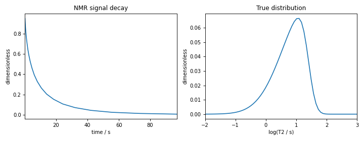
The following is the plot of the NMR signal decay as well as the corresponding true probability distribution.

>>> _, ax = plt.subplots(1, 2, figsize=(9, 3.5), subplot_kw={'projection': 'csdm'}) 
>>> ax[0].plot(data_object) 
>>> ax[0].set_xlabel('time / s') 
>>> ax[0].set_title('NMR signal decay') 
...
>>> ax[1].plot(true_t2_dist) 
>>> ax[1].set_title('True distribution') 
>>> ax[1].set_xlabel('log(T2 / s)') 
>>> plt.tight_layout() 
>>> plt.show() 

(png, hires.png, pdf)

_images/getting_started_relaxation-4.png

_images/null.png — Figure 7 The figure on the left is the NMR signal decay corresponding to \(T_2\) distribution shown on the right.¶

Generating the kernel¶

Import the T2 class and generate the kernel as follows,

>>> from mrinversion.kernel.relaxation import T2
>>> relaxT2 = T2(
...     kernel_dimension = data_object.dimensions[0],
...     inverse_dimension=dict(
...         count=64, minimum="1e-2 s", maximum="1e3 s", scale="log", label="log (T2 / s)"
...     )
... )
>>> inverse_dimension = relaxT2.inverse_dimension

In the above code, the variable relaxT2 is an instance of the T2 class. The two required arguments of this class are the kernel_dimension and inverse_dimension. The kernel_dimension is the dimension over which the signal relaxation measurements are acquired. In this case, this referes to the time at which the relaxation measurement was performed. The inverse_dimension is the dimension over which the T2 distribution is evaluated. In this case, the inverse dimension is a log-linear scale spanning from 10 ms to 1000 s in 64 steps.

Once the T2 instance is created, use the kernel() method of the instance to generate the relaxation kernel, as follows,

>>> K = relaxT2.kernel(supersampling=20)
>>> print(K.shape)
(25, 64)

Here, K is the \(25\times 64\) kernel, where the 25 is the number of samples (time measurements), and 64 is the number of features (T2). The argument supersampling is the supersampling factor. In a supersampling scheme, each grid cell is averaged over a \(n\) sub-grid, where \(n\) is the supersampling factor.

Data compression (optional)¶

Often when the kernel, K, is ill-conditioned, the solution becomes unstable in the presence of the measurement noise. An ill-conditioned kernel is the one whose singular values quickly decay to zero. In such cases, we employ the truncated singular value decomposition method to approximately represent the kernel K onto a smaller sub-space, called the range space, where the sub-space kernel is relatively well-defined. We refer to this sub-space kernel as the compressed kernel. Similarly, the measurement data on the sub-space is referred to as the compressed signal. The compression also reduces the time for further computation. To compress the kernel and the data, import the TSVDCompression class and follow,

>>> from mrinversion.linear_model import TSVDCompression
>>> new_system = TSVDCompression(K=K, s=data_object)
compression factor = 1.0416666666666667
>>> compressed_K = new_system.compressed_K
>>> compressed_s = new_system.compressed_s

Here, the variable new_system is an instance of the TSVDCompression class. If no truncation index is provided as the argument, when initializing the TSVDCompression class, an optimum truncation index is chosen using the maximum entropy method [5], which is the default behavior. The attributes compressed_K and compressed_s holds the compressed kernel and signal, respectively. The shape of the original signal v.s. the compressed signal is

>>> print(data_object.shape, compressed_s.shape)
(25,) (24,)

Statistical learning of relaxation parameters¶

The solution from a linear model trained with l1, such as the FISTA estimator used here, depends on the choice of the hyperparameters. To find the optimum hyperparameter, we employ the statistical learning-based model, such as the n-fold cross-validation.

The LassoFistaCV class is designed to solve the l1 problem for a range of \(\lambda\) values and determine the best solution using the n-fold cross-validation. Here, we search the best model using a 5-fold cross-validation statistical learning method. The \(\lambda\) values are sampled uniformly on a logarithmic scale as,

>>> lambdas = 10 ** (-7 + 6 * (np.arange(64) / 63))

Fista LASSO cross-validation Setup¶

Setup the smooth lasso cross-validation as follows

>>> from mrinversion.linear_model import LassoFistaCV
>>> f_lasso_cv = LassoFistaCV(
...     lambdas=lambdas,
...     inverse_dimension=inverse_dimension,
...     sigma=0.0008,
...     folds=5,
... )
>>> f_lasso_cv.fit(K=compressed_K, s=compressed_s)

The arguments of the LassoFistaCV is a list of the lambda values, along with the standard deviation of the noise, sigma. The value of the argument folds is the number of folds used in the cross-validation. As before, to solve the problem, use the fit() method, whose arguments are the kernel and signal.

The optimum hyperparameters¶

The optimized hyperparameters may be accessed using the hyperparameters attribute of the class instance,

>>> lam = f_lasso_cv.hyperparameters['lambda']

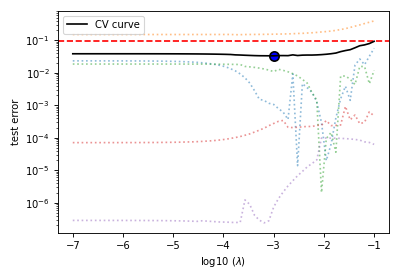
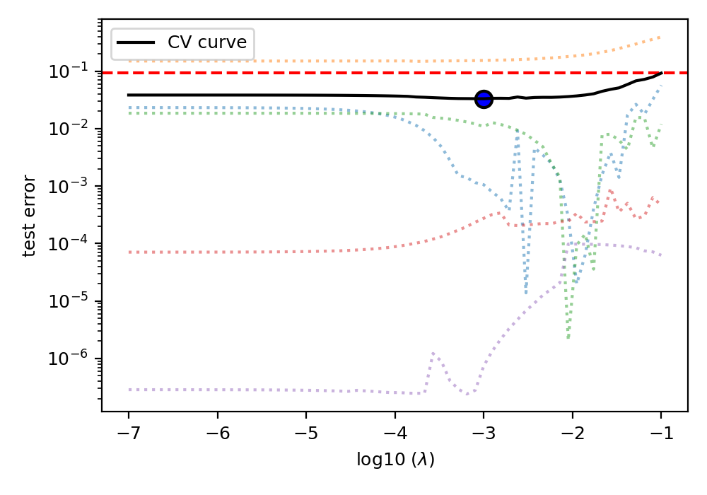
The cross-validation curve¶

The cross-validation error metric is the mean square error metric. You may plot this data using the cv_plot function.

>>> plt.figure(figsize=(5, 3.5)) 
>>> f_lasso_cv.cv_plot() 
>>> plt.tight_layout() 
>>> plt.show() 

(png, hires.png, pdf)

_images/getting_started_relaxation-12.png

The optimum solution¶

The best model selection from the cross-validation method may be accessed using the f attribute.

>>> f_sol_cv = f_lasso_cv.f  # best model selected using the 5-fold cross-validation

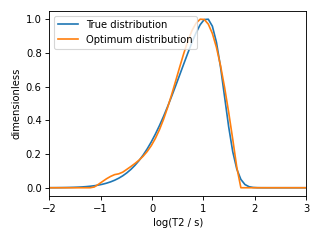
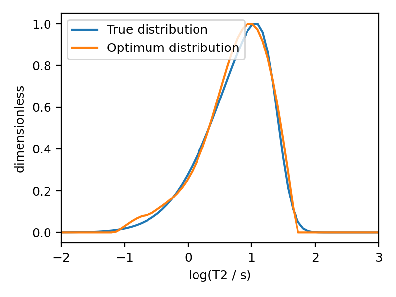
The plot of the selected T2 parameter distribution is shown below.

>>> plt.figure(figsize=(4, 3)) 
>>> plt.subplot(projection='csdm') 
>>> plt.plot(true_t2_dist / true_t2_dist.max(), label='True distribution') 
>>> plt.plot(f_sol_cv / f_sol_cv.max(), label='Optimum distribution') 
>>> plt.legend() 
>>> plt.tight_layout() 
>>> plt.show() 

(png, hires.png, pdf)

_images/getting_started_relaxation-14.png