Note
Go to the end to download the full example code.
Intermediary T2 distribution (Inverse Laplace)
The following example demonstrates the statistical learning based determination of the NMR T2 relaxation vis inverse Laplace transformation.
Before getting started
Import all relevant packages.
import csdmpy as cp
import matplotlib.pyplot as plt
import numpy as np

from mrinversion.kernel import relaxation
from mrinversion.linear_model import LassoFistaCV, TSVDCompression
Dataset setup
Load the dataset
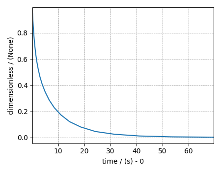
The variable signal holds the 1D dataset. For comparison, let’s
also import the true t2 distribution from which the synthetic 1D signal
decay is simulated.
datafile = f"{domain}/test2_t2.csdf"
true_t2_dist = cp.load(datafile)

plt.figure(figsize=(4.5, 3.5))
signal.plot()
plt.tight_layout()
plt.show()
Linear Inversion setup
Generating the kernel
kernel_dimension = signal.dimensions[0]

relaxT2 = relaxation.T2(
    kernel_dimension=kernel_dimension,
    inverse_dimension=dict(
        count=64, minimum="1e-2 s", maximum="1e3 s", scale="log", label="log (T2 / s)"
    ),
)
inverse_dimension = relaxT2.inverse_dimension
K = relaxT2.kernel(supersampling=20)
Data Compression
new_system = TSVDCompression(K, signal)
compressed_K = new_system.compressed_K
compressed_s = new_system.compressed_s

print(f"truncation_index = {new_system.truncation_index}")
compression factor = 1.0416666666666667
truncation_index = 24
Fista LASSO cross-validation
Create a guess range of values for the \(\lambda\) hyperparameters.
lambdas = 10 ** (-7 + 6 * (np.arange(64) / 63))

# setup the smooth lasso cross-validation class
f_lasso_cv = LassoFistaCV(
    lambdas=lambdas,  # A numpy array of lambda values.
    folds=5,  # The number of folds in n-folds cross-validation.
    sigma=sigma,  # noise standard deviation
    inverse_dimension=inverse_dimension,  # previously defined inverse dimensions.
)

# run the fit method on the compressed kernel and compressed data.
f_lasso_cv.fit(K=compressed_K, s=compressed_s)
The optimum hyper-parameters
print(f_lasso_cv.hyperparameters)
{'lambda': np.float64(0.0004159562163071843)}
The cross-validation curve
plt.figure(figsize=(4.5, 3.5))
f_lasso_cv.cv_plot()
plt.tight_layout()
plt.show()

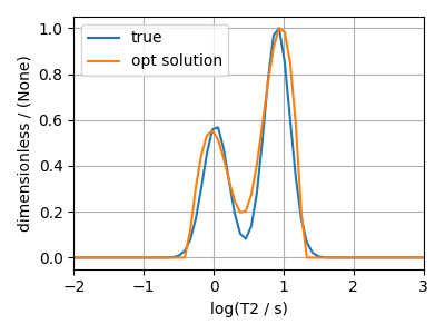
The optimum solution
sol = f_lasso_cv.f

plt.figure(figsize=(4, 3))
plt.subplot(projection="csdm")
plt.plot(true_t2_dist / true_t2_dist.max(), label="true")
plt.plot(sol / sol.max(), label="opt solution")
plt.legend()
plt.grid()
plt.tight_layout()
plt.show()
Residuals
residuals = f_lasso_cv.residuals(K=K, s=signal)
print(residuals.std())

plt.figure(figsize=(4.5, 3.5))
residuals.plot()
plt.tight_layout()
plt.show()
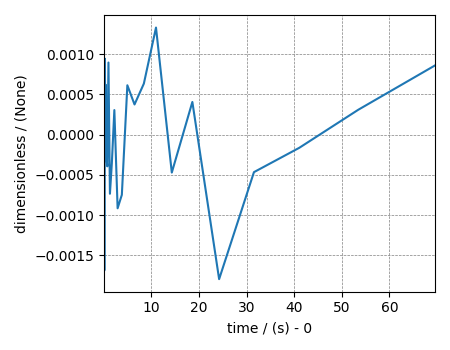
0.0007806697928656407
Total running time of the script: (0 minutes 0.809 seconds)