0.07 Li2O • 0.02 Al2O3 • 0.001 SnO2 • 0.91 SiO2 MAS-ETA

The following example is an application of the statistical learning method in determining the distribution of the Si-29 echo train decay constants in glasses.

Import all relevant packages.

import csdmpy as cp
import matplotlib.pyplot as plt
import numpy as np

from mrinversion.kernel import relaxation
from mrinversion.linear_model import LassoFistaCV, TSVDCompression
from csdmpy import statistics as stats

plt.rcParams["pdf.fonttype"] = 42  # For using plots in Illustrator
plt.rc("font", size=9)


def plot2D(csdm_object, **kwargs):
    plt.figure(figsize=(4, 3))
    csdm_object.plot(cmap="gist_ncar_r", **kwargs)
    plt.tight_layout()
    plt.show()

Dataset setup

Import the dataset

Load the dataset as a CSDM data-object.

# The 2D SE-PIETA MAS dataset in csdm format
domain = "https://www.ssnmr.org/sites/default/files/mrsimulator"
filename = f"{domain}/MAS_SE_PIETA_7Li_2Al_91Si_FT.csdf"
data_object = cp.load(filename)

# Inversion only requires the real part of the complex dataset.
data_object = data_object.real
sigma = 1194.356  # data standard deviation

# Convert the MAS dimension from Hz to ppm.
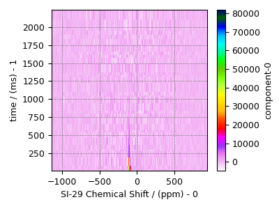
data_object.dimensions[0].to("ppm", "nmr_frequency_ratio")
plot2D(data_object)

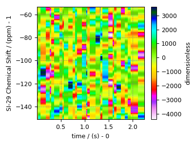
Prepping the data for inversion

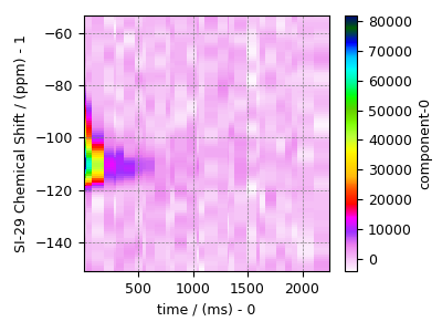
data_object = data_object.T
data_object_truncated = data_object[:, 1220:-1220]
plot2D(data_object_truncated)

Linear Inversion setup

Dimension setup

data_object_truncated.dimensions[0].to("s")  # set coordinates to 's'
kernel_dimension = data_object_truncated.dimensions[0]

Generating the kernel

relaxT2 = relaxation.T2(
    kernel_dimension=kernel_dimension,
    inverse_dimension=dict(
        count=32,
        minimum="1e-3 s",
        maximum="1e4 s",
        scale="log",
        label=r"log ($\lambda^{-1}$ / s)",
    ),
)
inverse_dimension = relaxT2.inverse_dimension
K = relaxT2.kernel(supersampling=20)
print(K.shape)

(32, 32)

Data Compression

new_system = TSVDCompression(K, data_object_truncated)
compressed_K = new_system.compressed_K
compressed_s = new_system.compressed_s

print(f"truncation_index = {new_system.truncation_index}")

compression factor = 2.1333333333333333
truncation_index = 15

Solving the inverse problem

FISTA LASSO cross-validation

# setup the pre-defined range of alpha and lambda values
lambdas = 10 ** (-4 + 5 * (np.arange(32) / 31))

# setup the smooth lasso cross-validation class
s_lasso = LassoFistaCV(
    lambdas=lambdas,  # A numpy array of lambda values.
    sigma=sigma,  # data standard deviation
    folds=5,  # The number of folds in n-folds cross-validation.
    inverse_dimension=inverse_dimension,  # previously defined inverse dimensions.
)

# run the fit method on the compressed kernel and compressed data.
s_lasso.fit(K=compressed_K, s=compressed_s)

The optimum hyper-parameters

print(s_lasso.hyperparameters)

{'lambda': 0.038075460212223716}

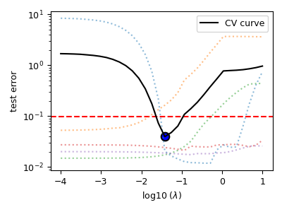
The cross-validation curve

plt.figure(figsize=(4, 3))
s_lasso.cv_plot()
plt.tight_layout()
plt.show()

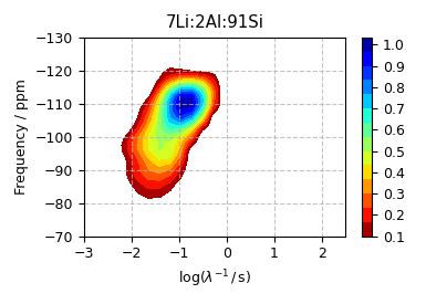
The optimum solution

f_sol = s_lasso.f

levels = np.arange(15) / 15 + 0.1
plt.figure(figsize=(3.85, 2.75))  # set the figure size
ax = plt.subplot(projection="csdm")
cb = ax.contourf(f_sol / f_sol.max(), levels=levels, cmap="jet_r")
ax.set_ylim(-70, -130)
ax.set_xlim(-3, 2.5)
plt.title("7Li:2Al:91Si")
ax.set_xlabel(r"$\log(\lambda^{-1}\,/\,$s)")
ax.set_ylabel("Frequency / ppm")
plt.grid(linestyle="--", alpha=0.75)
plt.colorbar(cb, ticks=np.arange(11) / 10)
plt.tight_layout()
plt.show()

The fit residuals

residuals = s_lasso.residuals(K=K, s=data_object_truncated)
plot2D(residuals)

The standard deviation of the residuals is

residuals.std()

<Quantity 1299.08377798>

Saving the solution

f_sol.save("7Li-2Al-91Si_inverse.csdf")  # save the solution
residuals.save("7Li-2Al-91Si-residue.csdf")  # save the residuals

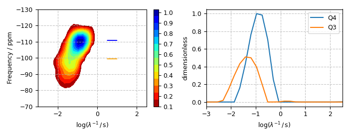
Analysis

# Normalize the distribution to 1.
f_sol /= f_sol.max()

# Get the Q4 and Q3 cross-sections.
Q4_coordinate = -110.7e-6  # ppm
Q3_coordinate = -99.3e-6  # ppm
Q4_index = np.where(f_sol.dimensions[1].coordinates >= Q4_coordinate)[0][0]
Q3_index = np.where(f_sol.dimensions[1].coordinates >= Q3_coordinate)[0][0]

Q4_region = f_sol[:, Q4_index]
Q3_region = f_sol[:, Q3_index]

Plot of the Q4 and Q3 cross-sections

fig, ax = plt.subplots(1, 2, figsize=(7, 2.75), subplot_kw={"projection": "csdm"})
cb = ax[0].contourf(f_sol, levels=levels, cmap="jet_r")
ax[0].arrow(1, Q4_coordinate * 1e6, -0.5, 0, color="blue")
ax[0].arrow(1, Q3_coordinate * 1e6, -0.5, 0, color="orange")
ax[0].set_ylim(-70, -130)
ax[0].set_xlim(-3, 2.5)
ax[0].set_xlabel(r"$\log(\lambda^{-1}\,/\,$s)")
ax[0].set_ylabel("Frequency / ppm")
ax[0].grid(linestyle="--", alpha=0.75)

ax[1].plot(Q4_region, label="Q4")
ax[1].plot(Q3_region, label="Q3")
ax[1].set_xlim(-3, 2.5)
ax[1].set_xlabel(r"$\log(\lambda^{-1}\,/\,$s)")
ax[1].grid(linestyle="--", alpha=0.75)

plt.colorbar(cb, ax=ax[0], ticks=np.arange(11) / 10)
plt.tight_layout()
plt.legend()
plt.savefig("7Li-2Al-91Si.pdf")
plt.show()

Mean and mode analysis

The T2 distribution is sampled over a log-linear scale. The statistical mean of the Q4_region and Q3_region in log10(T2). The mean T2 is 10**(log10(T2)), in units of seconds.

Q4_mean = 10 ** stats.mean(Q4_region)[0] * 1e3  # ms
Q3_mean = 10 ** stats.mean(Q3_region)[0] * 1e3  # ms

Mode the argument corresponding to the max distribution.

# index corresponding to the max distribution.
arg_index_Q4 = int(np.argmax(Q4_region))
arg_index_Q3 = int(np.argmax(Q3_region))

# log10(T2) coordinates corresponding to the max distribution.
arg_coord_Q4 = Q4_region.dimensions[0].coordinates[arg_index_Q4]
arg_coord_Q3 = Q3_region.dimensions[0].coordinates[arg_index_Q3]

# T2 coordinates corresponding to the max distribution.
Q4_mode = 10**arg_coord_Q4 * 1e3  # ms
Q3_mode = 10**arg_coord_Q3 * 1e3  # ms

Results

print(f"Q4 statistics:\n\tmean = {Q4_mean} ms,\n\tmode = {Q4_mode} ms\n")
print(f"Q3 statistics:\n\tmean = {Q3_mean} ms,\n\tmode = {Q3_mode} ms\n")
print(f"r_λ (mean) = {Q4_mean/Q3_mean}")
print(f"r_λ (mode) = {Q4_mode/Q3_mode}")

Q4 statistics:
        mean = 128.70911289809567 ms,
        mode = 107.71050560367647 ms

Q3 statistics:
        mean = 42.29792062171425 ms,
        mode = 38.0754602122236 ms

r_λ (mean) = 3.0429182098379792
r_λ (mode) = 2.828869434625967